

Does Technical Analysis Work? I Tested the Famous Chart Rules on 100 Years of Data
Tested on daily U.S. returns since 1928, the 1992 moving-average rules beat a same-exposure mix until 1986. Since publication, all ten trail buy and hold.
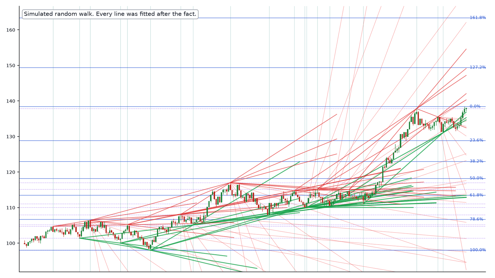
Search for technical analysis and you will find charts like the one below: candlesticks under a web of Fibonacci retracements, trendlines, fan lines and support levels, each one touching a turning point. The prices in this one are simulated. They come from a random walk, so nothing that happened on one day could tell you anything about the next, and every line was fitted after the fact. It took a few minutes to make it look like analysis.
That does not settle whether technical analysis works, because the question covers several different claims, and some of them have real evidence behind them. The most famous academic case for chart rules is a 1992 study by William Brock, Josef Lakonishok and Blake LeBaron, which found that simple moving-average rules on the Dow predicted returns over 90 years of data. So I took their ten moving-average rules, plus three popular ones, and ran them on daily U.S. stock market returns from 1928 to September 2026, as an investor would have had to: trading at the next close, paying costs, sitting in T-bills when out, and compared with the right benchmarks. Then I ran the same rules through a taxable account.
The short version
- Drawn chart patterns (head-and-shoulders, Fibonacci levels, candlesticks) have a weak or negative record as trading strategies in most tests that define them precisely.
- Mechanical moving-average rules did contain information before 1987. In my test, Brock et al.’s ten rules beat a static stock and T-bill mix with the same average stock exposure by a median 3.0 points a year from 1928 to 1986, after costs, with a one-day trading delay, and that result survives a test for searching many rules. Dropping the 1929-32 crash cuts it to 1.9 points.
- From 1993, after the study was published, every one of the ten rules trailed buy and hold, by 1.0 to 6.1 points a year, and their median edge over the same-exposure mix was about zero.
- The slower rules did cut the deepest losses, most of all in the 2000-02 and 2008-09 bear markets, and then missed much of the rebound. In a taxable account the frequent switching cost far more: for a $100,000 account from 1993 in the 32% bracket plus the 3.8% surtax, at today’s rates, the 200-day rule ended with $1.18 million after tax against $2.51 million for buy and hold.
- Trend following has better evidence as a diversified futures strategy than as a timing signal on one stock index. If you want it, buy it as a sized sleeve, ideally in a tax-advantaged account.
What counts as technical analysis
Technical analysis means forecasting from past prices and trading volume rather than from a company’s business. Under that label sit activities with very different evidence behind them:
| Approach | Example | What the evidence shows |
|---|---|---|
| Drawn chart patterns | Head-and-shoulders, triangles, Fibonacci retracements, candlesticks | Mostly negative once patterns are defined by a fixed rule |
| Mechanical timing rules | 200-day moving average, golden cross, RSI and MACD thresholds | Worked on old index data; faded after publication and costs |
| Cross-sectional momentum | Buy the stocks that rose most over the past year, sell the laggards | Large published literature, with crashes and real trading costs |
| Time-series momentum | Hold each futures market long or short according to its own trend | Positive across many markets and decades, in simulations net of fees |
| Order-flow analysis | Where stop-loss and take-profit orders cluster | Real mechanism behind some support and resistance in currencies |
It also helps to separate three claims that get run together. The first is that past prices carry some information about future returns. The second is that a particular rule captures enough of it to show up in a fair statistical test. The third is that an individual investor can profit from it after trading costs, taxes and competition from everyone else who has read the same study. The first can be true while the other two are false, and most of the argument about technical analysis is people defending the first claim and selling the third.
A random walk will draw you a convincing chart
Pattern-finding on charts is unreliable because noise produces patterns. A series with no memory at all still makes runs, reversals, double tops and channels, and the eye finds them most easily after the fact, when it can see where the price went next. The lines in the opening chart were placed at the swing highs and lows of the finished series, which no trader could have known in advance.
Real markets are more than random noise, and people can tell. In a 2010 online experiment, Jasmina Hasanhodzic, Andrew Lo and Emanuele Viola asked 78 people to pick the real price chart out of pairs in which the other chart was the same returns shuffled into random order. Across 8,015 guesses, they did it far more often than chance would allow.1 Real prices have structure that shuffling destroys, such as calm periods and turbulent ones that cluster together. Recognizing that texture is a different skill from knowing whether the next move is up or down, and the experiment did not test the second.
The 1992 study and what happened to it
Brock, Lakonishok and LeBaron tested 26 rules on the Dow Jones Industrial Average from 1897 to 1986: ten moving-average crossover rules, ten fixed-holding versions and six breakout rules. Days after a buy signal had higher average returns than days after a sell signal, and the gap was too large to come from several standard models of random prices.2 Two details matter for investors. The paper compared buy days with sell days and did not compare a strategy with buy and hold. It also left out trading costs; a later re-examination put the break-even cost of the rules at 0.39% per trade over the full sample and 0.22% for 1976-91.3
Ryan Sullivan, Allan Timmermann and Halbert White returned to the same data in 1999 with a much larger universe of 7,846 rules and a statistical test, White’s Reality Check, built to correct for having searched through so many. The best rule over 1897-1986 still passed. Then they looked forward: the rule that was best by the end of 1986 earned a mean return of 2.8% a year over 1987-96, with a p-value of 0.32, far from significant, and on S&P 500 futures from 1984 to 1996 they found no evidence that any of the rules beat the benchmark.4
Pierre Bajgrowicz and Olivier Scaillet took the same 7,846 rules through 2011 in 2012 with a different correction for false discoveries. For 1962-2011 they found no outperforming rules at all, even before trading costs. In the earlier periods, one-way costs of 16 to 70 basis points erased what the rules had earned, and they concluded that “an investor would never have been able to select ex ante the future best-performing rules.”5
Other tests point the same way. Franklin Allen and Risto Karjalainen let a genetic algorithm search for the best rules on the S&P 500 from 1928 to 1995 and reported that “after transaction costs, the rules do not earn consistent excess returns over a simple buy-and-hold strategy in the out-of-sample test periods.”6 Back in 1966, Eugene Fama and Marshall Blume found that small filter rules beat buy and hold on Dow stocks before costs, and Fama later summarized that floor traders’ minimum fees of about 0.1% a round trip were “sufficient to wipe out their advantage over buy-and-hold.”7 A 2007 survey by Cheol-Ho Park and Scott Irwin counted 56 positive, 20 negative and 19 mixed results among 95 modern studies, with profits found “at least until the early 1990s,” and listed the usual problems: data snooping, rules chosen after the fact, and hard-to-measure risk and costs.3
The best evidence for technical analysis
- Chart patterns can carry information. Andrew Lo, Harry Mamaysky and Jiang Wang wrote an algorithm to find ten classic patterns, including head-and-shoulders and double bottoms, in U.S. stocks from 1962 to 1996. Returns after a pattern were distributed differently from other returns for all ten patterns on Nasdaq and for seven of ten on NYSE and AMEX stocks. The authors added that “informativeness does not guarantee a profitable trading strategy”; they did not test trading profits or costs.8
- Price trends help forecast the market. Christopher Neely, David Rapach, Jun Tu and Guofu Zhou found that technical indicators forecast the monthly U.S. equity premium from 1950 to 2011, in and out of sample, as well as or better than standard economic variables. The two kinds of signal were complementary: price trends caught declines near business-cycle peaks, and economic variables caught recoveries near troughs.9
- A large reported anomaly. Yufeng Han, Ke Yang and Guofu Zhou applied a 10-day moving average to portfolios of stocks sorted by volatility from 1963 to 2009 and reported risk-adjusted returns of 9.3% to 21.8% a year, largest for the most volatile stocks.10 The portfolios were equal-weighted, traded daily and heavy in small stocks, and the paper reported costs only as break-even levels, roughly 29 to 112 basis points a trade depending on the portfolio. I could not find a published out-of-sample replication.
- A mechanism for support and resistance. Carol Osler at the Federal Reserve Bank of New York found that exchange rates bounced off the support and resistance levels published by six firms 60.8% of the time, against 56.2% for arbitrary levels.11 Her later work explained why: take-profit orders cluster at round numbers and stop-loss orders just beyond them, so prices tend to stall at round numbers and then run once they break through.12 Neither paper tested whether trading on the levels paid after costs.
- One famous chartist’s record held up. Alfred Cowles scored William Peter Hamilton’s Dow Theory editorials in the 1930s and concluded he lagged buy and hold. Stephen Brown, William Goetzmann and Alok Kumar re-scored them in 1998, measuring them against risk as well as return, and concluded that his calls over 1902-1929 “yield high Sharpe ratios and positive alphas.”13
- Professionals use it. In Lukas Menkhoff’s survey of 692 fund managers in five countries, 87% used technical analysis to some extent and 18% preferred it to other methods. It was their most important tool for forecasts a few weeks out.14
The drawn patterns themselves fare worse. Osler tested head-and-shoulders trading on 100 randomly chosen U.S. stocks from 1962 to 1993 and found it unprofitable.15 (The pattern did pay in currency tests for the Deutsche mark and yen, though not for four other exchange rates.16) Candlestick signals added no value on Dow stocks from 1992 to 2002.17 A test of Fibonacci retracements on stocks in the Dow 30, DAX 30 and Nasdaq 100 from 1968 to 2019 found prices no more likely to turn at Fibonacci levels than at random ones, and concluded the results “provide no support for the use of Fibonacci retracements.”18
I reran the famous rules on 100 years of daily data
The published tests mostly stop in 2011 or earlier and mostly ask whether a rule predicts returns. I wanted to know what the rules would have done for an investor since then, so I set the test up the way an investor would have to live with it.
- Data: daily returns of the whole U.S. stock market (the CRSP value-weighted index, which includes dividends) from Kenneth French’s data library, July 1926 to September 2026, with T-bill returns from the same source.19 Moving averages are calculated on a price index (dividends stripped out using Robert Shiller’s monthly S&P dividend yield), as chart readers use.20 The 200-day signal built this way agrees with one built from actual S&P 500 closing prices on 96.7% of trading days since 1928.
- Rules, fixed in advance: Brock et al.’s ten moving-average rules (five pairings of a 1, 2 or 5-day average with a 50, 150 or 200-day average, each with and without a 1% band); the 50/200-day golden cross; Meb Faber’s 10-month rule (in the market when the month-end price is above its 10-month average); and a 12-month trend rule (in the market when the past year’s return beat T-bills). When a rule is out, the money sits in T-bills.
- Trading: a signal computed at one day’s close is traded at the next day’s close, with a cost of 0.05% on each switch.
- Benchmarks: buy and hold, and a fixed mix of stocks and T-bills holding the rule’s average stock share. A rule that is in the market 70% of the time will usually trail buy and hold simply because stocks beat T-bills. The same-exposure mix asks whether the timing itself added anything.
- Uncertainty: 90% intervals from a block bootstrap, and White’s Reality Check across the rule set, the same test Sullivan, Timmermann and White used.
| Period | Buy and hold, per year | Median edge vs. buy and hold | Median edge vs. same-exposure mix |
|---|---|---|---|
| 1928-1986 (inside their sample) | 9.3% | +1.1 | +3.0 |
| 1933-1986 (without 1929-32) | 11.9% | -0.9 | +1.9 |
| 1987-1996 | 14.7% | -4.9 | -2.8 |
| 1993-2026 (after publication) | 10.9% | -2.0 | 0.0 |
| 2013-2026 | 14.8% | -3.5 | -1.3 |
Brock, Lakonishok and LeBaron’s ten moving-average rules on the CRSP U.S. market, traded at the next close with 0.05% per switch. Edges are differences in annual compound return, in percentage points. The Reality Check p-value is the chance that the best of the ten would look this good against the same-exposure mix if none of them had any edge (stationary bootstrap, 63-day mean blocks, 2,000 draws). Periods end September 30, 2026. Author’s calculation, ta_rules.py.
In the period Brock et al. studied, the rules worked in my test too, and by more than enough to survive the costs I charged. All ten beat the same-exposure mix, nine of them with intervals that exclude zero, and the Reality Check says the best of them was very unlikely to be luck. Against plain buy and hold the edge was smaller, from +0.3 to +1.8 points a year, and no interval excluded zero.
The Great Crash accounts for part of the early record. Dropping 1929-32 turns every rule’s edge over buy and hold negative, and the edge over the same-exposure mix shrinks to a median 1.9 points, with 3 of the 10 intervals excluding zero (Reality Check p = 0.047).
Stale prices are the reason for the one-day delay. Before electronic trading, many stocks in an index did not trade every day, so a daily index partly reflected old prices and today’s return partly predicted tomorrow’s. The correlation between one day’s market return and the next was 0.23 in 1962-86 and has been slightly negative since 1987; two days apart it was close to zero in both eras. A rule allowed to trade at the same close as its signal would capture that staleness, which no investor could have traded. Doing so raises the median edge over buy and hold for 1928-86 from 1.1 to 1.8 points a year. The next-close test in the table leaves most of that out.
After the study’s sample ended, the edge stopped showing up across the board. In Sullivan, Timmermann and White’s 1987-96 test window, all ten rules lagged both benchmarks. From 1993 on, every rule trailed buy and hold, and the median edge over the same-exposure mix was zero to one decimal place, with a Reality Check p-value of 0.53. The chart shows the 200-day rule decade by decade. After 1997 its edge over the same-exposure mix is positive in the decades that contain all of the 2000-02 or 2008-09 bear market (those ending from late 2002 to 2018) and mostly negative otherwise.
The rules most investors have heard of tell the same story since 1993:
| Rule, Jan 1993 to Sep 2026 | Return per year | Edge vs. same-exposure mix (90% range) | Worst drawdown |
|---|---|---|---|
| Buy and hold | 10.9% | n/a | -55% |
| 200-day moving average | 9.6% | +0.5 (-2.2 to +3.4) | -23% |
| 50/200-day golden cross | 10.3% | +1.1 (-1.6 to +3.9) | -34% |
| Faber 10-month | 9.9% | +0.8 (-2.0 to +3.8) | -22% |
| 12-month trend | 9.4% | +0.1 (-2.9 to +3.1) | -40% |
| 1/50-day crossover | 4.9% | -3.6 (-6.2 to -1.1) | -31% |
CRSP U.S. market and T-bills, next-close trading, 0.05% per switch, before taxes. A static mix holding 75% stocks and 25% T-bills over the same period had a worst drawdown of -43%. Author’s calculation, ta_rules.py.
None of the slower rules has an edge over the same-exposure mix that can be told apart from zero, and the fast 1/50-day rule lost to it by a margin that can. What the slower rules did deliver is shallower drawdowns, and here a static mix does not keep up: the 200-day rule’s worst loss was 23% against 43% for a fixed 75/25 portfolio. That protection came from a handful of episodes, and each one came with a bill:
| Decline | Market, decline | 200-day rule, decline | Market, next 12 months | 200-day rule, next 12 months |
|---|---|---|---|---|
| 1987 crash | -33% | -14% | +28% | +3% |
| 2000-02 bear market | -50% | -19% | +40% | +23% |
| 2008-09 bear market | -55% | -9% | +75% | +23% |
| 2020 COVID crash | -34% | -11% | +87% | +36% |
| 2022 bear market | -25% | -11% | +22% | +1% |
Market peak to trough on the CRSP U.S. index, then the 12 months after the trough. The golden cross, slower to react, took the full 34% loss in 2020. Author’s calculation, ta_rules.py.
Five declines make a small sample to build a strategy on. The 200-day rule got out early in all five, but in the 12 months after the 2020 low it gained 36% while the market gained 87%, and 23% against 75% after the 2009 low. The slower rules had a different problem: the golden cross and the 12-month rule took the full 34% loss in the fast 2020 crash.
I also ran a smaller version of the data-snooping problem. Out of a grid of 30 moving-average pairs, the best performer from 1928 to 1986 was a 2-day average crossing a 100-day average, which beat buy and hold by 2.1 points a year against a grid median of 1.1. From 1987 to 2026 it trailed buy and hold by 2.8 points a year, worse than the grid’s median rule, and ranked 21st of 30.
Momentum and trend following have a stronger record
The best evidence for using past prices comes from strategies that look nothing like a chart reader’s. Narasimhan Jegadeesh and Sheridan Titman found that buying the U.S. stocks with the highest returns over the past year and selling those with the lowest earned 1.31% a month before costs from 1965 to 1989, when held for three months.21 Robert Novy-Marx and Mihail Velikov found that a value-weighted momentum portfolio earned 0.68% a month after estimated trading costs (1.33% before), while higher-turnover strategies did not survive costs.22 Andrew Patton and Brian Weller found that typical mutual funds captured none of it after their own implementation costs.23
Time-series momentum, the strategy behind managed futures funds, follows each market’s own trend across dozens of futures contracts. Tobias Moskowitz, Yao Hua Ooi and Lasse Pedersen found that a market’s past 12-month return predicted its future returns across 58 futures and forward contracts, with the effect lasting about a year and then partly reversing.24 A simulation by Brian Hurst, Ooi and Pedersen back to 1880 across 67 markets earned 7.3% a year above T-bills after simulated trading costs and an assumed 2% management and 20% performance fee.25 That is a simulation, built by researchers at a firm that sells the strategy. Its edge comes from holding many markets long and short at once, which a single index moving in and out of T-bills cannot reproduce. Our managed futures guide covers the funds that run it, and the missing-best-days guide covers the critiques of trend timing on a single market.
Taxes turn a small pre-tax gap into a large one
Every exit from the market realizes a capital gain or loss. Gains on positions held one year or less are short-term and taxed as ordinary income.26 A loss is disallowed if you buy the same or a substantially identical security within 30 days before or after the sale; the loss is added to the cost basis of the new shares instead, and if the new shares are bought in an IRA it is lost for good.27 Above $200,000 of income for a single filer, or $250,000 for a married couple filing jointly, a 3.8% net investment income tax applies on top.28 A moving-average rule also earns T-bill interest while it is out, taxed every year as ordinary income, while a buy-and-hold investor defers tax on growth until selling.
I ran the rules through a taxable account starting with $100,000 in January 1993, applying today’s rates throughout for an investor in the 32% bracket who pays the 3.8% surtax: 35.8% on short-term gains, interest and nonqualified dividends, 18.8% on long-term gains and qualified dividends, with wash sales applied as the IRS applies them.
| $100,000 from Jan 1993 | Before tax | After tax, sold Sep 2026 |
|---|---|---|
| Buy and hold | $3.32M | $2.51M |
| 50/200-day golden cross | $2.72M | $1.57M |
| Faber 10-month | $2.45M | $1.32M |
| 12-month trend | $2.09M | $1.28M |
| 200-day moving average | $2.23M | $1.18M |
| 1/50-day crossover | $0.50M | $0.28M |
Single-lot model of a total-market fund, 0.05% per switch, dividends reinvested, each year’s tax paid the following April. Losses net and carry forward; the $3,000 ordinary-income offset and state taxes are ignored. Rates for 1993-2002 were different from today’s. With the 24% bracket and no surtax, buy and hold ends at $2.66 million and the 200-day rule at $1.39 million. Author’s calculation, ta_rules.py.
Before tax, the 200-day rule finished a third below buy and hold. After tax it finished at less than half. Most of its losing exits were followed by a re-entry within 30 days, which turns them into wash sales unless the investor re-enters through a different fund, and the IRS has never said which index funds count as substantially identical. In an IRA or 401(k) none of the tax drag applies, and the comparison falls back to the pre-tax tables above.
Studies of real traders, who use every method and not only charts, point the same direction. Brad Barber and Terrance Odean found that the most active fifth of 66,465 brokerage households earned 11.4% a year from 1991 to 1996 after commissions and spreads, against 17.9% for the market, before any taxes.29 In Taiwan, Barber and coauthors found that “less than 1% of the day trader population is able to predictably and reliably earn positive abnormal returns net of fees.”30 In Brazil, 97% of people who day traded equity futures for at least 300 days lost money.31 Our return-on-hassle guide covers those studies in more detail.
Why a backtest that worked can stop working
A strategy found by searching history is partly a measurement of that history. Test enough rules on one stretch of data and some will look excellent by chance; the best of them will look best partly because its luck was best. David Bailey, Jonathan Borwein, Marcos López de Prado and Jim Zhu showed how little searching it takes: “After trying only 7 independent strategy configurations, the expected maximum SR IS is 1 for a 2-year long backtest, while the expected SR OOS is 0.” (SR is the Sharpe ratio; IS and OOS mean in and out of sample.)32 And patterns that are real tend to shrink once published: across 97 return predictors, R. David McLean and Jeffrey Pontiff found returns 26% lower out of sample and 58% lower after publication.33
The lab below runs that process on markets where there is nothing to find. Each one is a random walk, so no rule has a real edge. It picks the best of up to 30 moving-average rules on the first ten years and then runs it, unchanged, on the next ten.
With the default settings, the backtest winner beats buy and hold by an average of 2.2 points a year in its own ten years and then trails it by 0.4 points a year live, beating it in 45% of markets. Searching more rules lifts the average backtest edge from -0.8 points with one rule to +2.2 with thirty, while the live edge stays between -0.4 and -0.8. The same thing happened with the real data above, where the best rule from 1928-86 went on to lose.
When a price rule can still make sense
- As a rule you will follow instead of panicking. An investor who would otherwise sell near a bottom and stay out for years may do better with a slow, written-down rule that gets back in. The evidence above prices that choice: shallower drawdowns, a lower long-run return, and in a taxable account a large tax bill. If you go this way, use a slow rule such as the 10-month or 200-day, hold it in an IRA or 401(k), and decide in advance which second fund you will use for re-entries in a taxable account.
- As risk control. Lowering exposure when markets turn volatile changes risk more reliably than it changes return. Our volatility targeting guide tests that idea directly.
- As a diversified trend sleeve. A managed futures fund applies trend rules across many markets long and short. That is the version with the strongest research behind it, and it fits as a sized slice of a portfolio rather than a switch on the whole thing.
- For the rare skilled trader. The Taiwan study found persistent winners, but they were a small minority of a population that lost in aggregate.30 Nothing in a chart tells you in advance whether you are one of them.
Test a rule before you trust it
Summitward's backtesting tool compares allocation strategies against historical returns, with drawdowns, recoveries and side-by-side results, so a rule's costs show up before real money is at stake.
Open backtestingFrequently asked questions
Does technical analysis work?
Some of it contained information in the past, and little of it pays an individual investor today. Simple moving-average rules beat a same-exposure mix of stocks and T-bills on U.S. data from 1928 to 1986, even after costs and a one-day trading delay. Since the rules were published they have trailed buy and hold, and after tax by a wide margin. Drawn chart patterns have a weaker record still.
Does the 200-day moving average beat buy and hold?
Not since 1993 in my test: it returned 9.6% a year against 10.9% for buy and hold through September 2026, before taxes, with a much smaller worst drawdown (23% against 55%). After tax in the 32% bracket plus the 3.8% surtax, at today’s rates, $100,000 grew to $1.18 million against $2.51 million. The missing-best-days guide covers the out-of-sample research on Faber’s 10-month version.
Do RSI and MACD work?
They are close relatives of the moving-average rules tested here: RSI compares recent gains with recent losses, and MACD is the gap between two moving averages. The large academic rule searches covered thousands of moving-average, breakout and filter variations of the same idea, and found that whatever worked on the Dow before the 1990s did not persist. Our crypto trend-following guide shows how indicator backtests fool their authors.
Do head-and-shoulders patterns work?
In U.S. stocks, the evidence says no. A Federal Reserve Bank of New York study of 100 stocks from 1962 to 1993 found head-and-shoulders trading unprofitable. Lo, Mamaysky and Wang found that the pattern carried some information about later returns, without showing that trading on it paid.
Do Fibonacci retracements work?
The largest test I found, on stocks in three major indexes from 1968 to 2019, found prices no more likely to turn at Fibonacci levels than at random levels, and trading on them did no better than trading on random levels.
Is Elliott Wave theory supported by evidence?
I could not find a rigorous peer-reviewed test of Elliott Wave forecasts on stock indexes. Wave counts are revised as prices unfold, which makes the method hard to test and its successes hard to separate from hindsight.
Do professional investors use technical analysis?
Many do. In a survey of 692 fund managers, 87% used it to some extent, mostly for forecasts a few weeks out, and 18% preferred it to other methods. Use is not evidence of profit; the same managers also face the costs and benchmarks that individual investors do.
Is technical or fundamental analysis better?
For most long-term investors, owning the whole market cheaply is a better default than either. Both are attempts to find mispriced securities, and both compete with professionals who have more data and lower costs. The factors with the longest research record, such as value and momentum, are systematic versions of each, available in low-cost funds.
Did FINRA end the pattern day trader rule?
In its old form, yes. FINRA’s amendments, effective June 4, 2026, replaced the day-trade count test and the $25,000 minimum equity requirement with intraday margin standards. Brokers have until October 20, 2027 to implement them, the $2,000 margin account minimum still applies, and firms can set stricter rules of their own.34 Easier access to day trading does not change the evidence on how day traders fare.
Key takeaways
- Lines drawn on a chart fit any price series after the fact, including a random one. Chart patterns, Fibonacci levels and candlesticks have weak or negative records as trading strategies when tested.
- Simple moving-average rules contained real information on old U.S. index data, even after costs and a one-day trading delay. From 1993, after publication, all ten of Brock et al.’s rules trailed buy and hold in my test, and their median edge over a same-exposure mix was about zero.
- Slow rules cut the worst drawdowns in slow bear markets and gave up much of the rebounds that followed.
- In a taxable account the switching is expensive. For one modeled investor in the 32% bracket paying the 3.8% surtax, at today’s rates from 1993, the 200-day rule ended with less than half the after-tax wealth of buy and hold.
- Trend following has its strongest evidence as a diversified futures strategy. Size it as a sleeve, preferably in a tax-advantaged account.
Related guides
- Missing the Market’s Best Days: the famous chart, trend timing and the research on both sides.
- Do You Need Managed Futures? for trend following across many markets.
- Growth Stocks vs. Systematic Momentum for cross-sectional momentum.
- The Engineer’s Guide to Systematic Investing for building rules worth following.
- The R² Trap, on another chart that randomness can draw.
- Why Macroeconomic Forecasts Are Not an Investment Strategy for the accuracy a market timer needs.
- Return on Hassle for the evidence on day trading.
Sources
- Jasmina Hasanhodzic, Andrew W. Lo and Emanuele Viola, “Is It Real, or Is It Randomized?: A Financial Turing Test”, working paper, February 2010. 78 subjects, 8,015 guesses; the randomized charts were the same returns in shuffled order.
- William Brock, Josef Lakonishok and Blake LeBaron, “Simple Technical Trading Rules and the Stochastic Properties of Stock Returns”, Journal of Finance 47(5), December 1992, 1731-1764 (abstract). Transaction costs were not included.
- Cheol-Ho Park and Scott H. Irwin, “What Do We Know About the Profitability of Technical Analysis?”, Journal of Economic Surveys 21(4), 2007, 786-826. The survey also reports Bessembinder and Chan’s (1998) break-even cost estimates for Brock et al.’s rules.
- Ryan Sullivan, Allan Timmermann and Halbert White, “Data-Snooping, Technical Trading Rule Performance, and the Bootstrap”, Journal of Finance 54(5), October 1999, 1647-1691. Table III and Section V for the 1987-96 results.
- Pierre Bajgrowicz and Olivier Scaillet, “Technical Trading Revisited: False Discoveries, Persistence Tests, and Transaction Costs”, Journal of Financial Economics 106(3), 2012, 473-491.
- Franklin Allen and Risto Karjalainen, “Using Genetic Algorithms to Find Technical Trading Rules”, Journal of Financial Economics 51(2), 1999, 245-271.
- Eugene F. Fama, “Efficient Capital Markets: A Review of Theory and Empirical Work”, Journal of Finance 25(2), 1970, 383-417, summarizing Fama and Blume, “Filter Rules and Stock-Market Trading,” Journal of Business 39(1), 1966.
- Andrew W. Lo, Harry Mamaysky and Jiang Wang, “Foundations of Technical Analysis: Computational Algorithms, Statistical Inference, and Empirical Implementation”, NBER Working Paper 7613, 2000; Journal of Finance 55(4), 2000, 1705-1765.
- Christopher J. Neely, David E. Rapach, Jun Tu and Guofu Zhou, “Forecasting the Equity Risk Premium: The Role of Technical Indicators”, Management Science 60(7), 2014, 1772-1791.
- Yufeng Han, Ke Yang and Guofu Zhou, “A New Anomaly: The Cross-Sectional Profitability of Technical Analysis”, Journal of Financial and Quantitative Analysis 48(5), 2013, 1433-1461.
- Carol L. Osler, “Support for Resistance: Technical Analysis and Intraday Exchange Rates”, Federal Reserve Bank of New York Economic Policy Review 6(2), July 2000.
- Carol L. Osler, “Currency Orders and Exchange Rate Dynamics: An Explanation for the Predictive Success of Technical Analysis”, Journal of Finance 58(5), 2003, 1791-1819 (working paper: FRBNY Staff Report 125).
- Stephen J. Brown, William N. Goetzmann and Alok Kumar, “The Dow Theory: William Peter Hamilton’s Track Record Reconsidered”, Journal of Finance 53(4), 1998, 1311-1333 (working paper version linked).
- Lukas Menkhoff, “The Use of Technical Analysis by Fund Managers: International Evidence”, Journal of Banking & Finance 34(11), 2010, 2573-2586 (discussion paper version linked). Survey of 692 managers in Germany, Switzerland, the U.S., Italy and Thailand, 2003-04.
- Carol L. Osler, “Identifying Noise Traders: The Head-and-Shoulders Pattern in U.S. Equities”, Federal Reserve Bank of New York Staff Report 42, 1998. Profits were negative but not statistically different from zero.
- P. H. Kevin Chang and Carol L. Osler, “Head and Shoulders: Not Just a Flaky Pattern”, FRBNY Staff Report 4, 1995; Economic Journal 109(458), 1999, 636-661.
- Ben R. Marshall, Martin R. Young and Lawrence C. Rose, “Candlestick Technical Trading Strategies: Can They Create Value for Investors?”, Journal of Banking & Finance 30(8), 2006, 2303-2323.
- Prodromos Tsinaslanidis, Francisco Guijarro and Nikolaos Voukelatos, “Automatic Identification and Evaluation of Fibonacci Retracements”, Expert Systems with Applications 187, 2022, 115893.
- Kenneth R. French, Data Library, Tuck School of Business: daily Fama/French factors (Mkt-RF) and monthly one-month T-bill returns, from the September 2026 CRSP update. Daily T-bill returns were rebuilt from the monthly series because the daily file rounds them to whole basis points.
- Robert J. Shiller, U.S. stock market data (ie_data.xls), monthly S&P Composite price and dividends; dividends after June 2026 carried forward.
- Narasimhan Jegadeesh and Sheridan Titman, “Returns to Buying Winners and Selling Losers: Implications for Stock Market Efficiency”, Journal of Finance 48(1), 1993, 65-91. The 12-month formation, 3-month holding strategy; gross of costs.
- Robert Novy-Marx and Mihail Velikov, “A Taxonomy of Anomalies and Their Trading Costs”, Review of Financial Studies 29(1), 2016, 104-147. Value-weighted momentum, net spread 0.68% a month (t = 2.45).
- Andrew J. Patton and Brian M. Weller, “What You See Is Not What You Get: The Costs of Trading Market Anomalies”, Journal of Financial Economics 137(2), 2020, 515-549.
- Tobias J. Moskowitz, Yao Hua Ooi and Lasse Heje Pedersen, “Time Series Momentum”, Journal of Financial Economics 104(2), 2012, 228-250.
- Brian Hurst, Yao Hua Ooi and Lasse Heje Pedersen, “A Century of Evidence on Trend-Following Investing”, Journal of Portfolio Management 44(1), Fall 2017. Simulated returns, January 1880 to December 2016.
- Internal Revenue Service, Topic no. 409, Capital gains and losses.
- Internal Revenue Service, Publication 550, Investment Income and Expenses, wash sales.
- Internal Revenue Service, Topic no. 559, Net investment income tax. The thresholds are not indexed for inflation.
- Brad M. Barber and Terrance Odean, “Trading Is Hazardous to Your Wealth: The Common Stock Investment Performance of Individual Investors”, Journal of Finance 55(2), 2000, 773-806.
- Brad M. Barber, Yong-Il Lee, Yu-Jane Liu and Terrance Odean, “The Cross-Section of Speculator Skill: Evidence from Day Trading”, Journal of Financial Markets 18, 2014, 1-24. Taiwan, 1992-2006.
- Fernando Chague, Rodrigo De-Losso and Bruno Giovannetti, “Day Trading for a Living?”, FGV EESP working paper 525, 2020 (not published in a journal). Brazilian equity futures, individuals who began day trading in 2013-15.
- David H. Bailey, Jonathan M. Borwein, Marcos López de Prado and Qiji Jim Zhu, “Pseudo-Mathematics and Financial Charlatanism: The Effects of Backtest Overfitting on Out-of-Sample Performance”, Notices of the American Mathematical Society, May 2014 (author copy linked).
- R. David McLean and Jeffrey Pontiff, “Does Academic Research Destroy Stock Return Predictability?”, Journal of Finance 71(1), 2016, 5-32.
- FINRA, Regulatory Notice 26-10, April 20, 2026, and “Day Trading” investor page.
- All backtest, drawdown, after-tax and simulation figures are our calculations, reproducible with the scripts and data in summitward-research/does-technical-analysis-work. Primary conventions: signals from a price index built from the CRSP total return and Shiller dividends; trades at the next close; 0.05% per switch; T-bills when out; same-exposure and same-volatility static mixes rebalanced daily with hindsight weights; stationary block bootstrap with 63-day mean blocks (250-day blocks and the Politis-White automatic choice give similar intervals).
More in Investing & Portfolio
Browse all investing & portfolio guidesGet new guides by email
Evidence-based, no jargon. At most two emails a month. Unsubscribe any time.
Try it in Summitward
See historical backtesting in action with your own financial data. Free to start, no credit card required.