

Minimum Volatility and Betting Against Beta: What 15 Years of USMV Show
Nov 2011-Aug 2026: a 78% stock, 22% T-bill mix set to USMV's volatility matched its return and drawdown. The low-beta anomaly, BAB, and when min vol fits.
In May 2023 I asked on my Engineer Investor account why minimum-volatility funds got so little attention. I had just put USMV in a three-fund experiment next to a 3x S&P 500 fund and a managed futures fund, and the academic case for low-risk stocks looked stronger than the interest in them.

From my Engineer Investor account, May 2023. Disclosure: I write both Summitward and the Engineer Investor account.
USMV now has almost fifteen years of live data, which is enough to answer the question with numbers. From November 2011 through August 2026 it compounded at 11.69% a year with 11.1% volatility. The total US market fund VTI compounded at 14.64% with 14.3% volatility. A portfolio of 78% VTI and 22% Treasury bills, rebalanced monthly, compounded at 11.83% with 11.1% volatility and a slightly deeper worst drawdown. Over the full window, USMV and that plain stock-and-cash mix finished in the same place with the same risk. The path matters, though. Through December 2019, USMV had matched VTI’s return, 14.33% a year against 14.35%, with less volatility. The whole gap opened from January 2020 on.
The academic record behind low-risk investing goes back to 1972 and spans more than 20 markets, and the reasons the effect might persist are plausible. The fund most people buy to capture it delivered the volatility reduction it promised and no measurable risk-adjusted gain over its live history. Both facts matter for deciding whether to own it.
Three strategies that share a name
“Low volatility” covers at least three different portfolios, and the evidence for one does not transfer automatically to the others.
| Approach | How it picks stocks | Example |
|---|---|---|
| Low-volatility sort | Ranks stocks on their own trailing volatility and buys the quietest | SPLV: about 100 S&P 500 stocks with the lowest 12-month volatility, weighted by inverse volatility1 |
| Minimum-variance optimization | Uses a covariance matrix to find the combination with the lowest predicted portfolio risk, so correlations matter as much as each stock’s volatility | USMV: tracks the MSCI USA Minimum Volatility Index2 |
| Betting Against Beta (BAB) | Buys low-beta stocks levered up to a beta of 1 and shorts high-beta stocks de-levered to a beta of 1 | An academic long-short factor; no retail fund implements it3 |
BAB is designed to isolate one question: are low-beta stocks underpriced relative to high-beta stocks? A long-only fund like USMV answers a different one: what is the least volatile basket of large US stocks I can hold? Its returns contain the full equity market at a beta well below 1, plus whatever tilts the optimizer produces.
Higher-beta stocks have not earned proportionally more
The Capital Asset Pricing Model says a stock’s expected return above the risk-free rate should be proportional to its beta, its sensitivity to the market:
Plot expected return against beta and you get a straight line, the security market line. A stock with a beta of 1.5 should earn 1.5 times the market premium. An investor who wants more expected return should hold the market and borrow to lever it; one who wants less should mix the market with cash.
The data have disagreed since the first tests. Black, Jensen and Scholes found in 1972 that the realized line for NYSE stocks from 1931 to 1965 was flatter than the CAPM predicts: low-beta stocks earned more than their beta implied and high-beta stocks earned less, with the slope turning negative in the 1957 to 1965 subperiod.4 Haugen and Heins reported in 1975 that over the long run, stock portfolios with lower variance in monthly returns had earned higher average returns than their riskier counterparts.5
The later literature extended the result across measures and markets:
- Total volatility. Baker, Bradley and Wurgler sorted US stocks into quintiles on trailing volatility from 1968 to 2008. A dollar in the lowest-volatility quintile grew to $59.55; a dollar in the highest fell to $0.58, before costs.6 Restricted to the 1,000 largest stocks, the gap narrows to $55.53 against $24.14.
- Idiosyncratic volatility. Ang, Hodrick, Xing and Zhang found that across 23 developed markets, stocks with the highest idiosyncratic volatility underperformed the lowest by 1.31% a month after controlling for market, size and value, and the effect was significant in each G7 country individually.7
- Global portfolios. Blitz and van Vliet measured a 12 percentage point annual CAPM alpha spread between global low-volatility and high-volatility deciles from 1986 to 2006, appearing separately in the US, Europe and Japan.8
- Optimized portfolios. Clarke, de Silva and Thorley built long-only minimum-variance portfolios from the 1,000 largest US stocks. From 1968 to 2009 they earned 5.37% a year over T-bills with 11.90% volatility, against 4.88% and 15.56% for the market: a Sharpe ratio of 0.45 against 0.31.9
I ran the simplest version of the test on the Ken French data library, which sorts US stocks into five value-weighted groups on their trailing five-year beta. From July 1963 through August 2026, the highest-beta quintile had 2.3 times the beta of the lowest but earned only 1.5 times its excess return. Its Sharpe ratio was 0.38 against 0.53, and its compound annual return, 11.4%, was lower than the second quintile’s 11.6%.
The line is flatter than the CAPM predicts; it is not flat, and it is not inverted, for value-weighted beta sorts. The low-beta quintile’s CAPM alpha was 1.65% a year with a t-statistic of 1.96, right at the edge of conventional significance. Sort on total variance instead and the result is stronger: the highest-variance quintile earned 5.6% a year over T-bills against 7.1% for the lowest, less in absolute terms despite more than twice the volatility.
Why the anomaly might persist
A pattern this old should have been traded away unless something stops investors from exploiting it or it is compensation for a risk the CAPM leaves out. There are three leading explanations of the first kind and two serious challenges of the second.
Leverage constraints
Suppose you want 120% of the market’s risk but cannot or will not borrow. The CAPM answer, lever the market portfolio, is unavailable, so you buy stocks with betas above 1 instead. Enough investors doing this bid up high-beta stocks and leave low-beta stocks cheap. Fischer Black showed in 1972 that restricted borrowing produces a flatter security market line in equilibrium.10 Frazzini and Pedersen formalized the idea in 2014 and derived the prediction that investors who can use leverage should buy low-beta assets and lever them, which is the BAB factor.3 A 2020 follow-up by Asness, Frazzini, Gormsen and Pedersen split the low-risk effect into a correlation component and a volatility component and found the correlation component, which the leverage story predicts, earned strong returns in the US and internationally and moved with margin debt.11
Benchmarks
Most professional money is judged against a cap-weighted index. A manager who buys low-beta stocks will trail badly in bull markets even if the portfolio has better risk-adjusted returns, and that tracking error is a career risk. Baker, Bradley and Wurgler argue this benchmarking stops institutions from arbitraging the anomaly.6 The same force answers my 2023 question, as the live record below shows.
Lottery demand
Investors pay up for stocks with a small chance of a very large gain. Bali, Cakici and Whitelaw sorted stocks on their largest single-day return in the prior month and found the top decile underperformed the bottom by more than 1% a month. Controlling for that lottery characteristic reversed the negative relation between idiosyncratic volatility and returns.12 Liu, Stambaugh and Yuan find the beta anomaly is concentrated among overpriced stocks with high idiosyncratic volatility and becomes insignificant once that is controlled for, which points to mispricing of speculative stocks.13
The risk-based challenges
Two papers argue the anomaly is compensation for risk that the standard CAPM test misses. Cederburg and O’Doherty show that the beta of a high-minus-low beta portfolio falls when the equity premium is high and rises with market volatility, which biases the standard unconditional alpha downward; with a conditional CAPM estimated by instrumental variables, the beta anomaly disappears.14 Schneider, Wagner and Zechner argue that low-risk anomalies reflect compensation for coskewness risk, and that controlling for skewness makes the alphas of both betting against beta and betting against volatility insignificant.15
None of these explanations has won. Leverage constraints and lottery demand both have supporting evidence and probably both contribute. For an investor, the useful conclusion is narrower: the too-flat security market line is well established, while the size of the return premium you can capture from it depends heavily on how the portfolio is built.
Betting Against Beta
Frazzini and Pedersen’s BAB factor is the most cited implementation. Each month it estimates every stock’s beta from one year of daily volatility and five years of correlation with the market, shrinks the estimates toward 1, and splits stocks at the median beta. Each side is weighted by beta rank. The low-beta side is levered and the high-beta side de-levered so both have a beta of 1, and the factor buys the first and shorts the second.3
The published results were strong. In US stocks from 1926 to March 2012, BAB had a Sharpe ratio of 0.78 and a three-factor alpha of 0.73% a month with a t-statistic of 7.39. The authors found positive BAB returns in 18 of 19 other developed equity markets, and the same pattern in Treasuries, corporate bonds and futures.3
The critique
Novy-Marx and Velikov’s 2022 paper, titled “Betting against betting against beta,” argues that three construction choices inflate those numbers.16 In their 2018 working paper, which spans 1968 to 2017:
- Rank weighting behaves like equal weighting. For each dollar in BAB, the strategy committed on average $1.05 to stocks in the bottom 1% of market capitalization.
- Levering the low-beta side and de-levering the high-beta side works like hedging with the equal-weighted market. Hedged that way, BAB had a Sharpe ratio of 1.26; hedged with the value-weighted market, 0.80.
- Mixing one-year volatility with five-year correlation does not produce a true market beta, which leaves the factor less market-neutral than it appears.
- Built with value weights, BAB earned 0.56% a month with a Sharpe ratio of 0.49, against 1.08 for the original in their sample. Its five-factor alpha fell to 0.24% a month, not statistically significant, because it loaded heavily on profitability (RMW) and conservative investment (CMA).
The published abstract concludes that BAB earns positive returns after transaction costs, but earns them by tilting toward profitability and investment.16
BAB since publication
AQR still publishes monthly BAB returns. I split the US series at January 2014, when the paper appeared in print.17
| US BAB factor | Mean/yr | Vol | Sharpe | Alpha, FF5 + momentum (t) |
|---|---|---|---|---|
| Dec 1930 to Dec 2013 | 8.25% | 11.4% | 0.72 | 2.55% (1.74), from Jul 1963 |
| Jan 2014 to Jul 2026 | 4.97% | 8.9% | 0.56 | 3.60% (1.57) |
Author’s calculation from AQR’s “Betting Against Beta: Equity Factors, Monthly” (USA column, downloaded 2026-09-29) and Ken French factors. The pre-2014 alpha starts in July 1963, when the five-factor data begin. Gross of trading costs. AQR revises its history on each update.
The average return fell by about 40% after publication, smaller than the 58% average decline in anomaly returns that McLean and Pontiff measured across 97 predictors.18 Volatility fell too, so the Sharpe ratio dropped by only about a fifth. The factor-adjusted alpha was 2.55% a year before 2014 and 3.60% after, and neither half is statistically significant on its own; over the full July 1963 to July 2026 sample it is 3.63% with a t-statistic of 2.84. Both periods show the loading Novy-Marx and Velikov describe: a profitability coefficient of 0.57 before 2014 and 0.44 since (t = 5.0), plus 0.30 on momentum since 2014.
BAB is not a smooth ride either. Its worst drawdown in the AQR data was 54.6%, from May 1998 to February 2000, when high-beta technology stocks soared. It lost 9.6% in 2023. BAB shorts the stocks attracting the most speculative money, so it loses most when that speculation is rewarded.
The closest retail product, and why it differs
The best-known US-listed fund that buys low-beta and sells high-beta stocks is BTAL, now the AGF U.S. Market Neutral Anti-Beta Fund. It holds about 200 low-beta stocks long and 200 high-beta stocks short, equal-weighted and dollar-neutral within sectors, at a 1.40% net expense ratio.19
Dollar-neutral is a different target from beta-neutral. On August 31, 2026, BTAL’s long book had a beta of 0.62 and its short book 1.34, so the fund carried roughly −0.7 of net market beta. It behaves like a short position in the stock market plus a low-beta tilt. That made it a strong hedge in 2022, when it gained 20.90%, and a costly one in bull markets: it lost 14.85% in 2023, and from November 2011 through August 2026 it compounded at −2.9% a year in my calculation. BAB levers the low-beta side up to cancel that market exposure; BTAL does not. Treat BTAL as a hedge with an anti-beta tilt, and do not use it as a way to own the BAB premium.
Where low volatility sits among the factors
The five-factor model sharpened a question about low volatility: is it a separate effect, or quality under another name? Fama and French concluded that positive exposures to RMW and CMA, the returns of profitable firms that invest conservatively, capture the high average returns of low-beta and low-volatility stocks.20 Novy-Marx reached a similar conclusion, finding defensive-equity performance explained by size, profitability and relative valuation.21 Blitz and Vidojevic disagree for volatility specifically: beta earns no premium with or without the new factors, and they conclude the low-risk anomaly is not explained by the five-factor model.22
USMV’s own returns lean toward the Fama-French reading. Regressed on the five factors plus momentum from November 2011 to August 2026, it had a market beta of 0.73, positive loadings of 0.28 on profitability (t = 5.0) and 0.23 on investment (t = 3.3), a small momentum tilt, and an annualized alpha of −0.37% (t = −0.26), with 79% of monthly variation explained. Against the market alone its alpha was +1.4% a year, with a t-statistic under 1. Once profitability and investment enter the regression, the remaining alpha is indistinguishable from zero.
Two more sensitivities matter for anyone holding it:
- Interest rates. Government bonds co-move most with bond-like stocks, which Baker and Wurgler identify as large, mature, low-volatility, profitable dividend payers.23 Over USMV’s live history, holding the market constant, a 1% monthly gain in the intermediate Treasury fund IEF went with USMV beating VTI by about 0.3 percentage points (t = 4.5). Blitz, van Vliet and Baltussen review the evidence and conclude that this rate exposure explains only a small part of the low-volatility alpha.24
- Valuation. Research Affiliates estimated in 2016 that an S&P-methodology low-volatility strategy returned 0.82% a year more than the market from 2005 to 2015, of which 1.65% a year came from low-volatility stocks becoming more expensive relative to the market.25 A factor that has gotten more expensive has borrowed from its future returns. Today the gap is small: on August 31, 2026, the MSCI USA Minimum Volatility Index traded at 23.7 times trailing earnings and 19.6 times forward earnings, against 25.8 and 20.1 for the MSCI USA.26
On the evidence, I would place minimum volatility with the defensive tilts, next to profitability, rather than with value and momentum as a separate source of return. Its optimizer is built to minimize risk; return is not in its objective at all.
How USMV is built
MSCI starts from the roughly 525 large and mid-cap stocks in the MSCI USA Index and uses the Barra optimizer and risk model to find the long-only portfolio with the lowest predicted total risk, subject to constraints.2 The main ones:
- No stock above the lower of 1.5% or 20 times its weight in the parent index, and none below 0.05%.
- Each sector within 5 percentage points of its parent weight.
- Exposure to style factors other than beta and residual volatility held within 0.25 standard deviations of the parent.
- Since August 2025, quarterly rebalancing (previously semiannual) with one-way turnover capped at 5% per review (previously 10%), keeping the same 20% annual turnover budget.
The constraints exist because covariance matrices are estimated, and an unconstrained optimizer will pile into whatever stocks look least correlated in the sample. They also explain holdings that surprise people. USMV had 33% of its assets in information technology on September 28, 2026, and its largest holding was Amphenol at 1.68%, followed by Nvidia and Microsoft.27 Minimum variance does not mean utilities and consumer staples; a technology stock that is weakly correlated with the rest of the basket can lower the portfolio’s risk.
USMV charges 0.15%, held 173 stocks on September 28, 2026, and managed about $23 billion.27 Its siblings follow the same method: ACWV (global, 0.20%), EFAV (developed ex-US, 0.20%) and EEMV (emerging markets, 0.25%), all launched October 18, 2011.28
Fifteen years of live data
| Nov 2011 to Aug 2026 | CAGR | Vol | Sharpe | Worst drawdown (monthly) |
|---|---|---|---|---|
| USMV | 11.69% | 11.1% | 0.91 | −19.1% |
| SPLV | 10.12% | 11.7% | 0.75 | −21.4% |
| VTI | 14.64% | 14.3% | 0.92 | −24.8% |
Author’s calculation, 178 months, from Yahoo Finance dividend-adjusted closes. Sharpe ratios use one-month T-bill returns from the Ken French data library. Drawdowns are measured on month-end values, which understate intra-month declines.
BlackRock’s own figures agree. Over the same period it reports USMV at 11.75% a year with 11.15% risk and a Sharpe ratio of 0.90, against 15.09%, 13.91% and 0.96 for the S&P 500, with 72% upside capture and 65% downside capture.29 At the June 30, 2026 quarter end, its standardized ten-year return was 9.59% against 15.49% for the MSCI USA.27
The calendar years show the trade the fund makes:
| Year | USMV | VTI | Difference |
|---|---|---|---|
| 2012 | 10.8% | 16.5% | −5.6 |
| 2013 | 25.1% | 33.4% | −8.4 |
| 2014 | 16.3% | 12.5% | +3.8 |
| 2015 | 5.4% | 0.4% | +5.1 |
| 2016 | 10.6% | 12.8% | −2.2 |
| 2017 | 18.9% | 21.2% | −2.3 |
| 2018 | 1.3% | −5.2% | +6.6 |
| 2019 | 27.7% | 30.7% | −3.0 |
| 2020 | 5.6% | 21.1% | −15.4 |
| 2021 | 20.8% | 25.7% | −4.8 |
| 2022 | −9.4% | −19.5% | +10.1 |
| 2023 | 10.3% | 26.0% | −15.7 |
| 2024 | 15.7% | 23.8% | −8.1 |
| 2025 | 7.6% | 17.1% | −9.4 |
| 2026 (Jan to Aug) | 8.6% | 13.5% | −4.9 |
Total returns from Yahoo Finance dividend-adjusted closes; difference in percentage points. Author’s calculation.
USMV beat VTI in four of fourteen full years: 2014, 2015, 2018 and 2022. Three things in that record deserve attention.
- It worked in the slow bear market. In 2022, when stocks fell on rising rates and valuations, USMV lost 9.4% against 19.5% for VTI.
- It barely helped in the fast one. From its February 2020 peak to the March 23 low, USMV fell 33.1% on daily closes against 35.0% for VTI. A covariance matrix estimated in calm markets does not know which stocks a pandemic will hit, and correlations jump toward 1 in a panic. For the full year, USMV then trailed the recovery by 15.4 points.
- Deep losses remain possible. MSCI’s index history shows a maximum drawdown of 47.2% from October 2007 to March 2009, against 55.4% for the MSCI USA.26 That period is before USMV existed and partly before the index launched in June 2008, so part of it is a backtest. Min vol is still an all-equity portfolio.
The pattern holds outside the US too. Over the same window EFAV compounded at 7.25% with 11.1% volatility against 8.19% and 14.4% for EFA, and EEMV at 5.06% and 12.5% against 5.67% and 16.9% for EEM. The international funds kept more of their parent’s return than USMV did, but none produced a statistically significant alpha, and EFAV lost slightly more than EFA in 2022.
Min vol against owning fewer stocks
Most people consider a min-vol fund because 100% stocks feels like too much risk. The simpler way to take less stock market risk is to own less of the stock market. That makes a VTI and T-bill mix with the same risk the correct benchmark for USMV, and the numbers are close to identical:
| Nov 2011 to Aug 2026 | CAGR | Vol | Sharpe | Worst drawdown |
|---|---|---|---|---|
| USMV | 11.69% | 11.1% | 0.91 | −19.1% |
| 78% VTI + 22% T-bills (volatility-matched) | 11.83% | 11.1% | 0.92 | −19.5% |
| 66% VTI + 34% T-bills (beta-matched) | 10.32% | 9.5% | 0.92 | −16.7% |
Hypothetical portfolios, rebalanced monthly, gross of trading costs and taxes, using one-month T-bill returns from the Ken French data library. The weights come from USMV’s realized volatility and its beta of 0.66 to VTI over the same window, so both use hindsight. Author’s calculation.
The two mixes differ because USMV is more volatile than its beta alone implies: the market explains only 72% of its monthly variation, and the rest is sector and factor tilt. Match on volatility and the mix earns the same return; match on beta and the mix gives up 1.4 points of return for less volatility and a smaller drawdown. On either basis, over this window, the optimizer added nothing a simple allocation could not reproduce.
The verdict depends on the end date. Stop the clock in December 2019 and USMV looks like the academic low-risk result in action: the market’s return at lower volatility, well ahead of any risk-matched mix. From January 2020 through August 2026 it compounded at 8.5% a year against 15.0% for VTI and 12.5% for the 78/22 mix, as a crash it barely cushioned gave way to a rally led by mega-cap growth stocks. About eight years of keeping pace followed by six and a half of lagging is ordinary for a factor strategy, and it is why fifteen years of live data cannot settle whether the low-risk premium survives. The pre-2020 tie also depends on the start month: across full calendar years 2012 to 2019, USMV compounded at about 14.2% a year against 14.6% for VTI.
The simple mix also has practical advantages. Its tracking error against the market is predictable, since it comes only from the cash weight. You can hold the safe portion in bonds or T-bills in whatever account is most tax-efficient. And its risk does not depend on a covariance forecast that can fail in a crash, as it did in March 2020.
MSCI makes the case for the opposite framing. For an investor with a fixed risk budget who wants more equity exposure, minimum-variance stocks let a portfolio move twice as much from bonds into equities as cap-weighted stocks for the same added risk, using global indexes,, which added about 0.7 percentage points a year from 2006 to 2020 in their analysis.30 That argument depends on low-risk stocks delivering better risk-adjusted returns than the market, which they did in the long academic samples and did not in USMV’s live record.
Levering the boring stocks
If low-beta stocks are underpriced because investors will not use leverage, the investor who will should lever them. In February 2024 I asked whether anyone had packaged that.
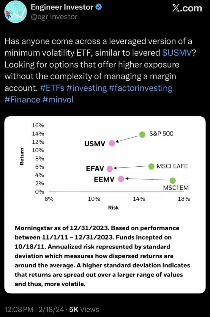
From my Engineer Investor account, February 2024. The attached chart shows Morningstar data from November 2011 to December 2023, as posted.
The product existed. UBS had launched the ETRACS 2x Leveraged MSCI US Minimum Volatility Factor TR ETN, ticker USML, in February 2021. It paid twice the quarterly compounded return of the MSCI USA Minimum Volatility index, minus a 0.95% annual tracking fee and a financing charge, and as an unsecured note it carried UBS credit risk. Almost no one bought it. UBS announced its redemption in July 2026, the last trading day was August 18, and holders received $47.256 per note. At the call, 100,000 notes were outstanding, about $4.7 million.31
Skipping it cost little over USMV’s live history. Levering USMV 1.28 times to match VTI’s volatility, financed at the T-bill rate plus 0.5%, would have compounded at 14.30% a year from November 2011 through August 2026 against 14.64% for VTI, with the same volatility. At T-bills plus 1.5%, roughly the lowest broker margin tiers, it drops to 13.98%; most retail margin accounts charge more. Levering the low-risk portfolio is the correct response to the leverage-constraint theory; in this window the low-risk portfolio had no edge to lever. The personal leverage guide covers the mechanics and the forced-selling risk.
Why min vol gets so little love
The answer to my 2023 question is in the calendar-year table. An investor who bought USMV in 2011 trailed a total market fund in ten of fourteen years, by 15 points or more twice, and ended with about 32% less money. Even with a Sharpe ratio equal to the market’s, that is hard to sit through while everyone around you owns the index. It is the benchmarking problem from the theory section applied to one person: a strategy can be defensible on risk-adjusted terms and still be abandoned because of when its underperformance arrives.
The long-run academic case for low-risk stocks is stronger than the live record of any single fund. Blitz, van Vliet and Baltussen report that a beta-neutral low-volatility factor earned a positive return in every decade from 1940 to 2018, with a Sharpe ratio of 0.65, though the authors work for Robeco, a low-volatility manager.24 Fifteen years is one draw, and since 2020 it has been dominated by a rally in large growth stocks that USMV held at well below market weight.
When min vol earns an allocation
My recommendation: for most DIY investors, skip minimum volatility and set risk with the stock-bond mix. If you want a defensive tilt anyway, keep it to a minority of the equity sleeve and pick an optimized fund such as USMV over a single-sort fund such as SPLV. Over the live period USMV beat SPLV in ten of fourteen years, with an alpha against it of 2.4% a year (t = 2.2). USMV’s index also limits how far each sector can drift from the market, which a single volatility ranking does not.
| Situation | Case for min vol |
|---|---|
| Young accumulator comfortable with market swings | Weak. Expected tracking error of several points a year for no expected gain in return. |
| Wants less total portfolio risk | Weak. Hold fewer stocks and more bonds or T-bills. The 78/22 mix above reproduced USMV. |
| Committed to a high equity allocation, for example a retiree funding spending from dividends and a separate pension or bond ladder | Moderate. The strongest conventional use. Lowers the volatility of the equity sleeve without changing the allocation, and brings a profitability and conservative investment tilt. |
| Sold in a past bear market and expects to again | Moderate, with a caveat. A 2022-style decline was halved; a 2020-style crash was not. Holding more bonds gives a more reliable cushion. |
| Portfolio concentrated in high-beta growth stock or employer equity | Moderate. The RMW and CMA tilt diversifies a growth-heavy book, though USMV still holds a third of its assets in technology. |
| Expects min vol to beat the market | Poor. Its objective is lower risk, and its live record trails the market by about 3 points a year. |
| Wants BAB exposure | No good retail option. BTAL is net short the market, and USML has been redeemed. |
If you do hold it, set the allocation and rebalance on a schedule. Adding min vol after a crash and dropping it after a rally is market timing with extra steps, and the calendar-year table shows how expensive a mistimed switch can be.
Key Takeaways
- The low-risk anomaly is well documented. In Ken French’s value-weighted beta quintiles from 1963 to 2026, the highest-beta stocks had 2.3 times the beta of the lowest and earned 1.5 times the excess return, with a Sharpe ratio of 0.38 against 0.53.
- BAB is the academic version, and its size is disputed. Frazzini and Pedersen reported a US Sharpe ratio of 0.78 from 1926 to 2012. Value-weighted, Novy-Marx and Velikov get 0.49 and an insignificant five-factor alpha. AQR’s US BAB series had a Sharpe ratio of 0.56 from 2014 to July 2026.
- USMV reduced risk and added no alpha. From November 2011 to August 2026 it compounded at 11.69% with 11.1% volatility against 14.64% and 14.3% for VTI. Sharpe ratios were 0.91 and 0.92, and its five-factor alpha was −0.37% a year.
- A stock-and-cash mix matched it. Over the same window, 78% VTI and 22% T-bills returned 11.83% with the same volatility, a result that uses hindsight to set the weights. Through 2019 USMV had matched VTI’s return; the gap opened from 2020 on.
- It protects better in slow declines than in crashes. USMV lost 9.4% in 2022 against 19.5% for VTI, but fell 33.1% in the February to March 2020 crash against 35.0%.
- Use it for a specific job. The case is strongest for an investor who will keep a high equity allocation and wants that sleeve to carry less risk. For everyone else, change the stock-bond mix.
Frequently Asked Questions
Is USMV a good investment?
It does what it is designed to do, which is hold US stocks with about three-quarters of the market’s volatility at a 0.15% expense ratio. From 2011 to 2026 it earned about 3 points a year less than the total market with a nearly identical Sharpe ratio. Whether that is good depends on whether you need lower-risk equities specifically or just lower risk, which a stock-bond mix provides more simply.
What is the difference between USMV and SPLV?
SPLV holds the 100 least volatile S&P 500 stocks weighted by inverse volatility, with no optimizer. USMV runs a covariance-based optimization across the MSCI USA with sector, weight and factor limits, and held a third of its assets in technology in 2026. From November 2011 to August 2026 USMV compounded at 11.69% against 10.12% for SPLV, with a Sharpe ratio of 0.91 against 0.75.
What is Betting Against Beta?
A long-short factor from Frazzini and Pedersen that buys low-beta stocks levered to a beta of 1 and shorts high-beta stocks de-levered to a beta of 1. It tests whether low-beta stocks are underpriced relative to high-beta stocks, and it is available as research data from AQR, not as a retail fund.
Is BTAL the same as Betting Against Beta?
No. BTAL is dollar-neutral, with equal dollars long low-beta and short high-beta stocks, so its net market beta is strongly negative. It behaves like a partial short on the stock market, which helped in 2022 and hurt in the 2023 and 2025 rallies.
Why does minimum volatility underperform in bull markets?
USMV’s beta to the total market was about 0.66 over its live history, so in a strong rally it participates in roughly two-thirds of the move. Recent rallies were led by high-beta mega-cap growth stocks, which the optimizer holds far below their index weights.
Does minimum volatility protect against crashes?
Partly. It halved the 2022 loss but fell 33.1% in the 2020 crash, only about two points less than the market. Its backtested index lost 47.2% in 2007 to 2009. It lowers equity risk; it does not replace bonds or cash.
Related Guides
- The ABCs of Systematic and Factor Investing for where low volatility sits among the other documented factors.
- HEDGEFUNDIE’s Excellent Adventure for the February 2023 UPRO, USMV and AQMIX portfolio and what was wrong with optimizing it on eleven years of data.
- RMW Explained: The Profitability Factor for the factor that absorbs most of USMV’s apparent alpha.
- Dividend Growth vs. Small-Cap Value for how dividend strategies load on low volatility and quality.
- Personal Leverage for margin, leveraged ETFs and forced selling.
- The Risk Parity Reality Check for the same leverage-constraint logic applied to bonds.
Sources
- Invesco S&P 500® Low Volatility ETF, summary prospectus dated December 19, 2025 (SEC EDGAR accession 0001193125-25-325659). sec.gov
- MSCI, “MSCI Minimum Volatility Indexes Methodology,” July 2025, including Appendix VIII on the changes effective August 2025. msci.com
- Andrea Frazzini and Lasse Heje Pedersen, “Betting Against Beta,” Journal of Financial Economics 111(1), 2014, 1–25. doi.org
- Fischer Black, Michael C. Jensen and Myron Scholes, “The Capital Asset Pricing Model: Some Empirical Tests,” in M. Jensen (ed.), Studies in the Theory of Capital Markets, Praeger, 1972, 79–121. efalken.com
- Robert A. Haugen and A. James Heins, “Risk and the Rate of Return on Financial Assets: Some Old Wine in New Bottles,” Journal of Financial and Quantitative Analysis 10(5), 1975, 775–784. Finding as summarized in Blitz, van Vliet and Baltussen (2020), p. 46. doi.org
- Malcolm Baker, Brendan Bradley and Jeffrey Wurgler, “Benchmarks as Limits to Arbitrage: Understanding the Low-Volatility Anomaly,” Financial Analysts Journal 67(1), 2011, 40–54. Dollar figures from the authors’ manuscript. nyu.edu
- Andrew Ang, Robert J. Hodrick, Yuhang Xing and Xiaoyan Zhang, “High Idiosyncratic Volatility and Low Returns: International and Further U.S. Evidence,” Journal of Financial Economics 91(1), 2009, 1–23. nber.org
- David Blitz and Pim van Vliet, “The Volatility Effect,” Journal of Portfolio Management 34(1), 2007, 102–113. doi.org
- Roger Clarke, Harindra de Silva and Steven Thorley, “Minimum-Variance Portfolio Composition,” Journal of Portfolio Management 37(2), 2011, 31–45. Extends their 2006 JPM paper, “Minimum-Variance Portfolios in the U.S. Equity Market.” doi.org
- Fischer Black, “Capital Market Equilibrium with Restricted Borrowing,” Journal of Business 45(3), 1972, 444–455. doi.org
- Cliff Asness, Andrea Frazzini, Niels Joachim Gormsen and Lasse Heje Pedersen, “Betting Against Correlation: Testing Theories of the Low-Risk Effect,” Journal of Financial Economics 135(3), 2020, 629–652. doi.org
- Turan G. Bali, Nusret Cakici and Robert F. Whitelaw, “Maxing Out: Stocks as Lotteries and the Cross-Section of Expected Returns,” Journal of Financial Economics 99(2), 2011, 427–446. nber.org
- Jianan Liu, Robert F. Stambaugh and Yu Yuan, “Absolving Beta of Volatility’s Effects,” Journal of Financial Economics 128(1), 2018, 1–15. doi.org
- Scott Cederburg and Michael S. O’Doherty, “Does It Pay to Bet Against Beta? On the Conditional Performance of the Beta Anomaly,” Journal of Finance 71(2), 2016, 737–774. doi.org
- Paul Schneider, Christian Wagner and Josef Zechner, “Low-Risk Anomalies?” Journal of Finance 75(5), 2020, 2673–2718. doi.org
- Robert Novy-Marx and Mihail Velikov, “Betting Against Betting Against Beta,” Journal of Financial Economics 143(1), 2022, 80–106. Construction details and figures from the November 2018 working paper. doi.org; working paper
- AQR Capital Management, “Betting Against Beta: Equity Factors, Monthly,” data through July 2026, downloaded September 29, 2026. aqr.com
- R. David McLean and Jeffrey Pontiff, “Does Academic Research Destroy Stock Return Predictability?” Journal of Finance 71(1), 2016, 5–32. doi.org
- AGF U.S. Market Neutral Anti-Beta Fund (BTAL), fact sheet as of August 31, 2026, and prospectus dated October 27, 2025. Calendar-year returns from the prospectus. agf.com
- Eugene F. Fama and Kenneth R. French, “Dissecting Anomalies with a Five-Factor Model,” Review of Financial Studies 29(1), 2016, 69–103. doi.org
- Robert Novy-Marx, “Understanding Defensive Equity,” NBER Working Paper 20591, 2014. nber.org
- David Blitz and Milan Vidojevic, “The Profitability of Low-Volatility,” Journal of Empirical Finance 43, 2017, 33–42. doi.org
- Malcolm Baker and Jeffrey Wurgler, “Comovement and Predictability Relationships Between Bonds and the Cross-Section of Stocks,” Review of Asset Pricing Studies 2(1), 2012, 57–87. doi.org
- David Blitz, Pim van Vliet and Guido Baltussen, “The Volatility Effect Revisited,” Journal of Portfolio Management 46(2), 2020, 45–63. eur.nl
- Rob Arnott, Noah Beck, Vitali Kalesnik and John West, “How Can ‘Smart Beta’ Go Horribly Wrong?” Research Affiliates, February 2016. PDF
- MSCI, “MSCI USA Minimum Volatility Index (USD)” factsheet, August 31, 2026, net returns. msci.com
- iShares MSCI USA Min Vol Factor ETF (USMV), product page and holdings file read September 29, 2026; fact sheet as of June 30, 2026. ishares.com
- iShares, “iShares Minimum Volatility ETFs” product brief, data as of August 31, 2026. ishares.com
- Harshad Jain and Mehdi Alighanbari, “Escaping to Equities for Yield,” MSCI blog, June 10, 2021. msci.com
- UBS ETRACS, USML product page and snapshot; UBS press releases “UBS Announces Redemption of Seven ETNs” (July 16, 2026) and “UBS Announces Call Settlement Amounts for Seven ETNs” (August 17, 2026). etracs.ubs.com
- Summitward calculations: fund returns from Yahoo Finance dividend-adjusted daily closes, factor, portfolio and T-bill returns from the Ken French data library (through August 2026), and AQR BAB returns. Script, data and printed output: summitward-research
Author disclosure
Summitward has no business relationship with BlackRock, MSCI, Invesco, AGF, UBS, AQR or any firm mentioned here and receives no compensation from them. Figures labeled as the author’s calculation are historical measurements over the stated window, not forecasts, and the hypothetical mixes are gross of trading costs and taxes. Nothing here is investment advice.
More in Investing & Portfolio
Browse all investing & portfolio guidesGet new guides by email
Evidence-based, no jargon. At most two emails a month. Unsubscribe any time.
Try it in Summitward
See portfolio factor analysis in action with your own financial data. Free to start, no credit card required.