

HEDGEFUNDIE's Excellent Adventure: The Whole Strategy Is a Bet on One Number
TMF has compounded at -6.34% a year since 2009. The 55/45 UPRO/TMF strategy works until stock-bond correlation crosses about +0.4, and nobody can tell you in advance where that line sits.
Direxion’s 3x long Treasury fund, TMF, launched in April 2009. Its average annual return since then is -6.34%. Compounded across seventeen years, $10,000 invested at launch is worth about $3,200 today.1 It is 92.89% below its 2020 peak, and it set that low in May 2026, about two months ago.
TMF is the defensive half of the most discussed leveraged portfolio in DIY investing. HEDGEFUNDIE’s Excellent Adventure pairs it with UPRO, a 3x S&P 500 fund, at 55/45, rebalanced quarterly. The thread that launched it ran past 3,000 posts. The strategy has its own acronym, its own follow-up thread, and a decade of arguments attached to it.
Most writing about HFEA falls into two camps. One reprints a spectacular backtest and explains how to rebalance. The other says leveraged ETFs decay and should never be held overnight. The first is credulous and the second is wrong on the mechanics. Neither tells you how to decide.
The short version
HFEA’s entire edge comes from stock-bond diversification raising the portfolio’s risk-adjusted return enough to justify levering it. Work out where that stops being true and you get a specific number: on reasonable assumptions, once the stock-bond correlation rises above roughly +0.4, the 55/45 mix delivers a worse risk-adjusted return than simply holding an unlevered S&P 500 fund, while carrying 300% gross exposure and paying financing on two turns of it. The strategy has no mechanism for noticing which regime it is in. And that breakeven point moves between roughly -0.3 and +0.85 depending on three parameters nobody can observe in advance.
What HFEA is
An anonymous Bogleheads user posted the strategy in February 2019, starting at 40% UPRO and 60% TMF. In August 2019 the allocation moved to 55/45 on the reasoning that equities drive the returns and the original mix held too much Treasury exposure. A second thread continues the discussion.2
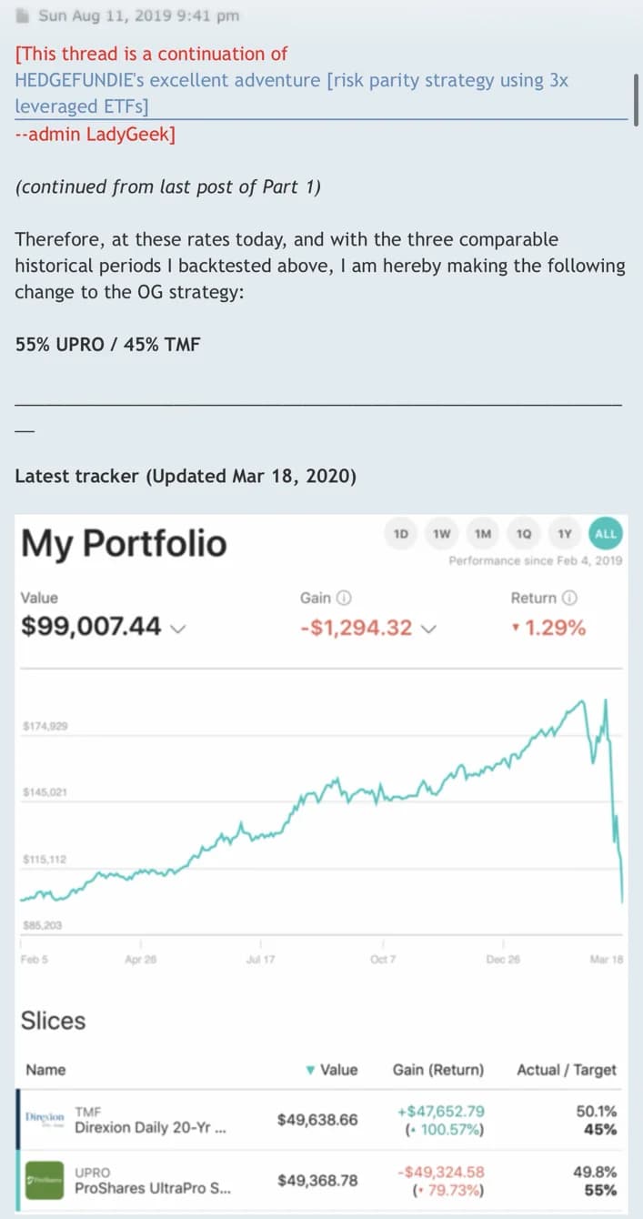
From the Part II thread. The tracker is dated March 18, 2020.
That tracker is worth sitting with. Thirteen months in, after peaking near $175,000, the account was at $99,007 against $100,000 invested. The hedge did what it was supposed to do, with TMF up 100.57% while UPRO fell 79.73%, and the portfolio still gave back everything. It is an early warning that a hedge working directionally is a different thing from a portfolio being safe.
The economics of the allocation are easy to state and easy to underestimate. Each dollar buys:
| Allocation | Equity exposure | Long Treasury exposure | Gross |
|---|---|---|---|
| 55/45 UPRO/TMF | 165% | 135% | 300% |
| 40/60 UPRO/TMF (original) | 120% | 180% | 300% |
| 43/57 UPRO/EDV | 129% | 57% | 186% |
Where to go for the implementation
This guide argues about whether the strategy makes sense. For how to actually run it, John Williamson’s write-up at Optimized Portfolio is the most thorough treatment anywhere: fund alternatives, rebalancing mechanics, and where to hold it. He has also run the strategy with his own money since October 2019 and posts quarterly updates, which is real evidence of a kind no backtest provides, and he discloses both his holdings and his referral relationships. He reaches a different conclusion than I do, which is exactly why he is worth reading alongside this. Find him at @optimizedport.
Three times your money goes into two of the most rate-sensitive assets available, one of which has a duration measured in decades. “Leveraged 60/40” undersells the concentration by a wide margin.
The idea underneath it is sound
Before the criticism, the strategy deserves its due, because the core insight is correct and most of its critics never engage with it.
Long-run compound growth for a levered position is approximately
where is the excess return over financing, the volatility, the leverage, and the financing spread. The variance penalty grows with the square of exposure, so growth rises with leverage to a peak and then falls. That peak sits at , which the Merton share guide works through for a single asset.
Both the growth expression and the optimum are Thorp’s, whose equations 7.2 and 7.3 give exactly this form with the financing rate subtracted inside the numerator.3 The distinction matters here more than almost anywhere: the numerator is the return in excess of what the leverage costs, so a rising short rate lowers the optimal leverage directly.
Put equities alone into that formula at a 5% excess premium and 15% volatility and the growth-optimal leverage is 2.22x. Thorp’s own worked example, using an 11% expected return, 15% volatility, and a 6% financing rate, lands on the same 2.22. A 3x equity fund is already past the point where more leverage helps compound growth. That is the real argument against holding 100% UPRO, and it has nothing to do with the word “decay.”
Now combine two imperfectly correlated assets. Diversification lowers portfolio volatility without lowering the mean proportionally, which raises the Sharpe ratio, which raises the leverage that maximizes growth. Using long Treasuries at a 2% term premium and 10% volatility against those same equities, at a 55% equity weight:
| Stock-bond correlation | Mix Sharpe | Versus unlevered equities | Growth-optimal leverage |
|---|---|---|---|
| -0.6 | 0.55 | +66% | 8.3x |
| -0.4 | 0.48 | +43% | 6.2x |
| -0.2 | 0.43 | +28% | 5.0x |
| 0.0 | 0.39 | +17% | 4.1x |
| +0.2 | 0.36 | +8% | 3.5x |
| +0.5 | 0.33 | -2% | 2.9x |
| +0.8 | 0.30 | -10% | 2.5x |
Read the last column. At a correlation of -0.4, the growth-optimal leverage for this mix is 6.2x, so running 3x is genuinely conservative. HEDGEFUNDIE’s instinct, that you should diversify first and lever the better portfolio rather than concentrate in the higher-returning one, is right, and it is the conclusion the personal leverage guide reaches from a different direction.
What daily reset actually does
The standard objection is that leveraged ETFs mechanically bleed value, so holding them is irrational. That is too strong. A 3x fund resets daily, which makes its multi-day return path-dependent: in a steady trend, daily compounding causes it to beat three times the index’s cumulative return, and in a choppy, directionless market it lags badly. Avellaneda and Zhang derived the exact relationship and validated it across 56 leveraged funds; the holder carries negative exposure to realized variance, and the sign of the leverage multiple does not change that.4 The cost is a function of how much the underlying moved around, not of how long it was held.
FINRA’s 2009 notice on these products has the clearest illustration anyone has produced. Between December 2008 and April 2009, a 3x leveraged financial-services ETF fell 53% while its underlying index gained 8%. Over the same window a 2x leveraged oil index ETF fell 6% while its index rose 2%.5 The index in that example was the Russell 1000 Financial Services Index, and the matching 3x inverse fund fell 90% over the same stretch. FINRA’s conclusion was that daily-reset leveraged and inverse ETFs “typically are unsuitable for retail investors who plan to hold them for longer than one trading session, particularly in volatile markets.”
UPRO’s own history shows the other side. ProShares reports its annualized NAV return since the June 2009 inception at 33.50%, against 15.42% for the S&P 500 total return index.6 That is 2.17 times the index’s compound rate rather than three times it, and the shortfall is financing and variance drag showing up in live data. Note also which direction the error runs in the popular version of this claim. The often-repeated line that UPRO delivered five times the index is true only of terminal wealth over one particular window, and multiples of cumulative wealth grow without bound with the holding period, so they describe the end date rather than the fund.
The strategy was designed when leverage was nearly free
A 3x fund borrows two turns of exposure for every turn of your capital. Relative to three times the index’s return, what it gives up is two turns of financing plus its expense ratio. That number is not a constant, and it moved a long way after 2019.
| Period | Short rate | Structural drag on 3x exposure |
|---|---|---|
| 2009 to 2015 | about 0.15% | 1.19% per year |
| 2021 | about 0.05% | 0.99% per year |
| 2023 to 2024 | about 5.2% | 11.29% per year |
| Mid 2026 | about 4.0% | 8.89% per year |
The strategy was written in February 2019 and refined through a period when this cost was close to one percent a year. It now runs closer to nine. Turn that around and it becomes a hurdle: at a 4% short rate and a 13% mix volatility, the underlying portfolio has to earn about 5.5% a year in excess return before the levered version breaks even against cash. At a 16% mix volatility the hurdle is about 6.8%.
None of this appears in a backtest that ends in 2018, and none of it is visible in the strategy’s design, which fixes leverage at 3x regardless of what borrowing costs.
The published literature got here first. Asness, Frazzini and Pedersen made the academic case for levered risk parity in 2012, reporting a higher Sharpe ratio than both the market and a 60/40 across an 85-year sample.7 Their headline results borrow at the risk-free rate. Anderson, Bianchi and Goldberg replicated the study and charged what borrowing actually costs. Levered risk parity beat 60/40 by 210 basis points a year over 1926 to 2010 on the original assumptions; with realistic borrowing costs that margin fell to 29 basis points and lost all statistical significance, and once trading costs were added, 60/40 won.8 Levered risk parity also underperformed across the whole 1946 to 1982 stretch.
To their credit, Asness and his coauthors anticipated the obvious objection that their result is an artifact of the bond bull market, and answered it: their sample starts in 1926 and contains a near-complete round trip in bond yields, alongside a near doubling of equity valuations, which if anything tilts the period toward equities. That is a fair response, and it does not address the financing-cost objection, which is the one that survives.
The leverage-aversion mechanism underneath all of this is contested too. Novy-Marx and Velikov show that the betting-against-beta result depends on a rank-weighting scheme that quietly equal-weights, committing about $1.05 per dollar invested to stocks in the smallest 1% of the market. They concede the strategy still earns positive returns after trading costs, but those returns carry no significant alpha against a five-factor model, and the evidence for the funding-constraint mechanism itself turns out to be an artifact of a non-standard beta estimator.9 None of that makes diversifying before levering wrong. It does mean the edge being levered is smaller and less certain than the strategy’s popular telling suggests.
The bet nobody priced
Look again at the table. As correlation rises, the Sharpe advantage shrinks, and at some point it reaches zero. On these assumptions that happens at a correlation of about +0.43. Past that point, an HFEA holder is carrying 300% gross exposure, paying financing on two turns of it, absorbing the variance penalty of two daily-reset 3x funds, and receiving a worse risk-adjusted return than someone who bought an S&P 500 index fund and did nothing.
The growth-optimal leverage tells the same story from another angle. At a correlation of -0.3 it is 5.5x, so 3x leaves room. At +0.5 it is 2.9x, so 3x is at the ceiling. At +0.8 it is 2.5x, and 3x is over it. HFEA runs 3x in all three cases. Nothing in the strategy observes the regime.
This is not a theoretical worry about a distant tail. It describes the 2020s. Drag the correlation slider below and watch the verdict change, or use the two regime buttons to flip between the world the backtest was run in and the world that followed it.
The breakeven is unknowable
Here is the part that should give any prospective HFEA investor pause. That +0.43 breakeven is not a constant. It depends on inputs that cannot be measured in advance, only assumed, and it moves a great deal when they change.
| Assumption changed | Correlation at which diversification stops paying |
|---|---|
| Long Treasuries have no term premium | -0.27, so it never pays at any plausible correlation |
| 1% term premium | +0.05 |
| Long Treasury volatility of 15% | +0.06 |
| Long Treasury volatility of 12% | +0.26 |
| Base case above | +0.43 |
| Equity premium of 4% rather than 5% | +0.63 |
| 3% term premium | +0.85 |
Three unobservable parameters, and the answer swings across almost the entire correlation range. If long Treasuries carry no term premium, levering them alongside equities never improves risk-adjusted return, no matter how negative the correlation goes. If they carry three points of term premium, the strategy survives almost anything.
Treat the specific figures as illustrative, because they follow from parameters I chose. The robust finding is the shape: the breakeven sits somewhere in a band running from roughly -0.3 to +0.85, its position depends on things you have to guess, and the strategy’s entire case lives inside that uncertainty. A backtest cannot resolve this, because a backtest reports one draw from the distribution of parameters rather than the distribution.
The backtest that recruited everyone
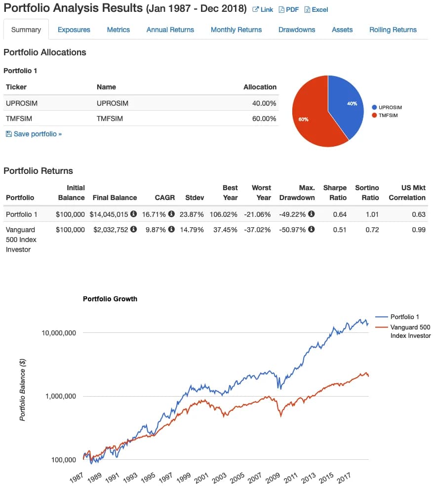
The simulated backtest circulated with the original thread, built from reconstructed UPRO and TMF series rather than fund data.
$100,000 becoming $14 million is a persuasive picture. The arithmetic holds up: 16.71% compounded for 32 years does give $14.04 million, and the 9.87% on the Vanguard 500 line is right for 1987 through 2018 once you subtract the fund’s expenses from the index.
Two things about it deserve more attention than the terminal value.
The first is the maximum drawdown of -49.22%, which is shallower than the S&P 500’s own -50.97% over the same window. A portfolio running 300% gross exposure showing less drawdown than its unlevered underlying is the entire risk-parity claim in one number. It is also precisely the claim that stopped holding.
The second is the start date. January 1987 begins the test near the top of a 35-year decline in long yields and excludes the 1970s and early 1980s bond bear market completely. The backtest contains no episode of the regime that would break the strategy, which is why it looks so good, and why it could not have warned anyone.
2022 was the out-of-sample test
In 2022, inflation forced rapid tightening, real and nominal yields rose, equity valuations compressed, and long-duration Treasuries fell hard. Both engines failed at once.
| 2022 | Since inception | Maximum drawdown | |
|---|---|---|---|
| UPRO | -56.80% | +33.50% per year | -76.82% (Feb to Mar 2020) |
| TMF | -72.80% | -6.34% per year | -92.89% (peak Mar 2020, low May 2026) |
The 2022 figures come from the funds’ own SEC filings.10 Running the actual 55/45 portfolio with quarterly rebalancing over that year gives about -64.2%, with a within-year drawdown near -67%. Measured from its December 2021 peak to the October 2023 trough, the strategy fell about -70.8%, and as of the end of July 2026 it remains roughly 37% below that peak, more than four and a half years later. Financing costs also rose through 2022, so the hurdle the leverage had to clear went up while the assets fell.
The deeper problem is in the second column. TMF has lost more than half its value across its entire seventeen-year life, including the tail end of the greatest bond bull market on record. Its trailing ten-year return is about -18% per year. The strategy’s defensive sleeve has not been a steady ballast that had one bad year. It has been a persistent drag held for its behavior in crises, and it set its all-time low two months ago.
Does EDV fix TMF?
A variant developed by MotoTrojan, who posts as @hml_compounder on X, swaps TMF for EDV, Vanguard’s extended-duration Treasury fund, at roughly 43/57.11 EDV holds long-dated Treasury STRIPS, is unlevered, and charges 0.05% against TMF’s 0.90%.1
It is a real improvement on several axes. Gross exposure falls from 300% to about 186%. There is no daily reset on the bond sleeve, so no variance penalty from it and no dependence on swap counterparties. Costs drop by most of a percentage point.
What it does not change is the thing that matters. EDV is still an extremely long-duration nominal bond fund whose value falls when long yields rise, and swapping it in leaves every parameter in the sensitivity table untouched. If the term premium on long Treasuries is thin and the correlation regime is positive, the EDV version fails for the same reason at a slower speed. It is the better implementation of the same bet.
I made the same mistake, with different tickers
In February 2023 I ran a mean-variance optimization in Portfolio Visualizer to design what I called a hedge-fund-style portfolio, looking for maximum return at a given volatility. It landed on roughly equal thirds of UPRO, USMV, and AQMIX.
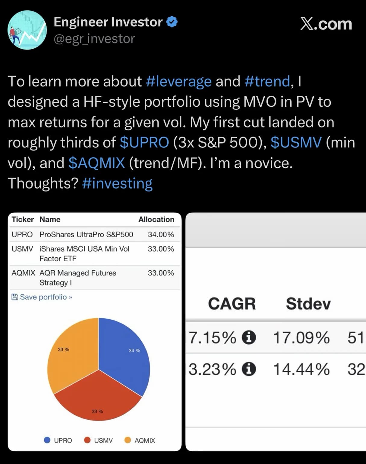
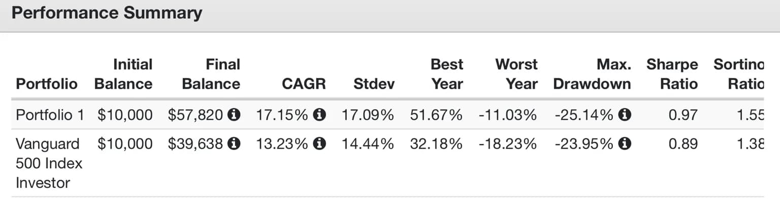
From my Engineer Investor account, February 2023. Disclosure: I write both Summitward and the Engineer Investor account.
The result looked excellent. A 17.15% compound return against 13.23% for the S&P 500, a higher Sharpe ratio, and a shallower maximum drawdown. I posted it and asked for criticism.
The criticism I gave myself in the same thread was the right one: the data only ran back to 2012, so I was optimizing on a US equity bull market. Work out how long that window was and the problem shows up in the numbers themselves. Growing $10,000 to $57,820 at 17.15% takes 11.1 years, or about 133 months. Every one of them came from the same regime.
There is a number for how much data an optimizer would actually need. DeMiguel, Garlappi and Uppal tested fourteen optimization models across seven datasets and found that none consistently beat naive equal weighting out of sample. Their calibrated estimate of the window required for sample-based mean-variance to reliably win is around 3,000 months for a 25-asset portfolio, which is 250 years.12 A three-asset problem needs less than that, and 133 months of a single regime is not in the neighborhood either way. What I had produced was a description of 2012 to 2023 with three tickers attached.
Three specific things were wrong with it, and they generalize:
- The optimizer had nothing to learn from. Optimizers fit the sample they are given. Over 2012 to 2023, the answer to what maximized return per unit of volatility was always going to be levered US equities plus whatever smoothed the ride. Michaud named the failure mode in 1989: mean-variance optimizers are, in his phrase, “estimation-error maximizers,” because they systematically overweight whatever assets happen to have the most flattering estimated inputs, and those are the assets whose estimates are most likely to be wrong.13
- It was more equity-concentrated than it looked. UPRO at 34% contributes 102% equity exposure, and USMV is a long-only US equity fund, so the portfolio carried about 135% US equity. Minimum volatility is an equity factor rather than a separate asset class, and the record since bears that out: from its October 2011 inception through July 2026, USMV compounded at 11.71% with 13.41% volatility against 14.95% and 16.72% for the S&P 500, a Sharpe ratio of 0.75 against 0.80. It delivered the lower volatility it advertises without converting it into a risk-adjusted advantage. In the February 2020 crash it fell 33.1% against the index’s 33.7%, a cushion of about seventy basis points in the fastest bear market on record. Novy-Marx goes further and shows that defensive-equity performance is explained once you control for size, profitability, and relative valuation, while the reverse does not hold.14
- Two-decimal weights implied precision that was not there. Small changes in estimated inputs move optimized weights a great deal, which the MPT guide covers directly.
The one part I would defend is the instinct behind AQMIX. A managed futures sleeve can go short bonds in a rising-rate trend and long commodities in an inflationary one, which is the adaptive behavior TMF structurally cannot provide. Whether that is worth its cost is a real question, and the managed futures guide works through it. Note that AQR currently reports AQMIX at a 3.09% gross and 3.09% net expense ratio with a 1.25% adjusted figure, where the adjustment removes financing and short-dividend expense.15 Those excluded costs are economically real, so 1.25% is not the cost of ownership.
The live record is the part worth internalizing before building a portfolio around trend following. AQMIX has returned 4.07% a year since its January 2010 inception against 1.45% for its T-bill benchmark, with 9.96% volatility, which is a Sharpe ratio of 0.26.15 The century-long simulation that made the case for trend following reports a net-of-fee Sharpe of 0.76 across 1880 to 2016, and the paper is explicit that those returns are simulated and the fees hypothetical. The academic time-series momentum factor reports a gross Sharpe above one, though Huang and coauthors later showed that asset-by-asset regressions find little evidence of the effect, that the pooled t-statistic fails bootstrap critical values, and that the strategy performs about as well as one built on the historical sample mean, which requires no predictability at all.16 Sixteen years of real money in a flagship fund run by two of the authors of that century paper produced roughly a third of the backtested risk-adjusted return. The fund did exactly what it was built for in 2022, gaining 35.4%, after seven consecutive calendar years from 2015 to 2021 that cumulatively lost money while equities roughly tripled.
The experiment was worth running. It was not a discovery.
Sizing a sleeve you can survive
If you have read this far and still want to try a levered sleeve, start by deciding how much of your wealth can sit inside it. The historical compound return does not answer that.
Work backwards from the loss you could absorb:
Someone who could tolerate a 5% hit to household wealth, assuming an 80% sleeve drawdown, gets 6.25% of investable assets. That is a different conversation from “what percentage should I allocate,” and it is the one worth having. UPRO has already delivered a 76.82% drawdown once, in about a month.
There is evidence on how badly this goes. Morningstar tracks the gap between what funds return and what the average dollar invested in them actually earns. Over the ten years to December 2024 the overall gap was 1.2 percentage points a year, and it widened with volatility: the least-volatile quintile of funds gave up 0.4 points a year while the most volatile gave up 2.0. Inside the alternatives category, the grouping closest to a leveraged or managed-futures sleeve, the most-volatile quintile gave up 11.0 points a year.17 Read that as a warning about the category rather than a precise tax; a 2026 rebuttal in the same journal family argues the headline gap conflates genuine mistiming with an accounting artifact and puts the true timing cost far lower. The ordering by volatility is the part worth keeping.
Also worth settling before you start rather than during a drawdown:
- Recovery arithmetic. A 60% loss needs a 150% gain to get back. An 80% loss needs 400%.
- Account location. Quarterly rebalancing between two volatile funds generates short-term gains in a taxable account.
- A written policy. Target weights, rebalancing rule, maximum sleeve size, and the conditions under which you would decide the thesis was wrong. Written in advance, because the point of writing it is that you will not want to follow it later.
- What would falsify it. If your answer is a sustained positive stock-bond correlation, check whether you would actually notice, and what you would do about it.
What most people should do instead
Almost nobody needs 3x funds to reach their goals, and the people who could survive one are generally the people who least need the extra risk.
If the appeal is capital efficiency rather than the leverage itself, that is available in far more robust forms. Return-stacked and capital-efficient funds provide roughly constant notional exposure without a daily reset, which the return stacking guide covers, and packaged risk-parity products handle the leverage inside a fund with disclosed limits rather than in your brokerage account, which the risk parity guide assesses. If the appeal is diversification against equity risk, which risk you are hedging is the subject of the bonds guide, and the answer determines whether nominal duration is the right tool at all.
How Summitward helps
Summitward does not recommend leveraged portfolios and has no HFEA preset. Two things it does are relevant if you are considering one.
The portfolio page runs a factor regression and a correlation matrix on your actual holdings, which is where a sleeve like this stops being abstract. A 10% HFEA position is a 30% gross addition to your balance sheet, and seeing the resulting equity beta and correlation structure alongside the rest of your portfolio is more informative than looking at the sleeve alone.
The retirement planner answers the question that decides it: whether the sleeve changes your probability of funding the plan. If a strategy raises your median outcome and leaves your success probability unchanged, it is entertainment. If it lowers the success probability, the historical compound return is beside the point.
Frequently asked questions
Is HEDGEFUNDIE’s Excellent Adventure a good strategy?
Its underlying principle is sound: diversify first, then lever the better portfolio, rather than concentrating in the highest-returning asset. Its implementation converts that principle into a bet on three unobservable parameters, and it holds a fixed 3x leverage whether the growth-optimal figure is 6x or 2.5x. For most investors the answer is no, and for the few it might suit, only as a small and explicitly loss-tolerant sleeve.
Do leveraged ETFs always lose money over time?
No. Daily reset makes returns path-dependent rather than uniformly negative. In a sustained trend a 3x fund beats three times the index’s cumulative return, which is why UPRO returned about 33.50% a year since 2009 against 15.42% for the index, which is 2.17 times the index’s compound rate rather than three times it. In choppy markets it lags badly, and FINRA documented a 3x fund falling 53% while its index rose 8% over five months. Both outcomes come from the same mechanism.
Why did HFEA fall so much in 2022?
Inflation caused equities and long-duration Treasuries to fall together, which removes the diversification the strategy depends on, while rising short rates raised the cost of the leverage. UPRO fell 56.80% and TMF fell 72.80% in the same calendar year, and the 55/45 portfolio fell about 64%.
Is the UPRO and EDV version better?
It is a better implementation. Gross exposure drops from about 300% to 186%, the bond sleeve has no daily reset or swap counterparties, and costs fall by most of a percentage point. It leaves the underlying macroeconomic bet unchanged, so it fails in the same conditions, more slowly.
How much should I put in it if I want to try?
Size it from the loss you can absorb rather than from a target allocation. Divide the household loss you could tolerate by the sleeve drawdown you assume. Tolerating a 5% household hit at an 80% assumed drawdown implies roughly 6% of investable assets, and UPRO has already delivered a 76.82% drawdown in about one month.
Key takeaways
- The defensive sleeve has been the problem. TMF has compounded at -6.34% a year since its April 2009 inception, turning $10,000 into roughly $3,200. It sits 92.89% below its 2020 peak and set that low in May 2026.
- The principle is right and the implementation is a guess. Levering a diversified portfolio beats concentrating in one asset, and 3x on equities alone is already past growth-optimal. Whether 3x on the mix is conservative or reckless depends on the regime.
- There is a breakeven correlation. On reasonable assumptions, past about +0.4 the levered mix delivers worse risk-adjusted returns than an unlevered S&P 500 fund while carrying 300% gross exposure.
- That breakeven cannot be measured in advance. It swings from -0.27 to +0.85 across plausible assumptions about the term premium, bond volatility, and equity premium.
- The famous backtest could not have warned anyone. It starts in January 1987, excludes the last bond bear market entirely, and reports a maximum drawdown shallower than the S&P 500’s own.
- Size the sleeve from the loss you can absorb. Tolerable household loss divided by assumed sleeve drawdown, which for most people lands in the single digits as a percentage of investable assets.
Related guides
- Korea’s 2x Single-Stock ETFs applies the same daily-reset arithmetic to a single stock at 117% volatility, with the measured nine-week result.
- The Risk Parity Reality Check the conceptual parent of this strategy, and why packaged products beat doing it yourself.
- The Merton Share the one-asset version of the growth-optimal leverage math used here.
- Personal Leverage margin mechanics, forced selling, and how daily-reset funds compare to borrowing directly.
- Are Bonds Still Good Diversifiers? which risk bonds actually hedge, and what changed in 2022.
- Do You Need Managed Futures? the adaptive alternative to a permanently long duration sleeve.
Sources
- Fund data from stockanalysis.com , retrieved July 29, 2026. TMF inception April 16, 2009; average annual return since inception -6.34%; expense ratio 0.90%. The cumulative figure in the text is compounded from that annualized rate. Maximum drawdown of -92.89% from a March 2020 peak, with the low on May 19, 2026, from Total Real Returns . EDV 0.05% and USMV 0.15% expense ratios from the same source.
- HEDGEFUNDIE, “HEDGEFUNDIE’s excellent adventure [risk parity strategy using 3x leveraged ETFs]” , Bogleheads forum, February 2019, and the Part II thread . The tracker image above is from Part II and is dated March 18, 2020.
- FINRA, Regulatory Notice 09-31 , June 11, 2009. The example covers December 1, 2008 to April 30, 2009 on the Russell 1000 Financial Services Index, and the oil example uses the Dow Jones U.S. Oil & Gas Index.
- Thorp, E. O. (2006). The Kelly Criterion in Blackjack, Sports Betting, and the Stock Market. In Handbook of Asset and Liability Management , Elsevier. Equations 7.2 and 7.3 give the levered growth rate g(f) = r + f(m − r) − s²f²/2 and the optimum f* = (m − r)/s². His worked example for the S&P 500 at m = 11%, s = 15%, r = 6% gives f* = 2.22.
- Avellaneda, M., & Zhang, S. (2010). Path-Dependence of Leveraged ETF Returns. SIAM Journal on Financial Mathematics, 1(1), 586–603 . Preprint: math.nyu.edu . Their equation 10 shows the holder of a leveraged ETF has negative exposure to realized variance regardless of the sign of the leverage multiple, validated across 56 leveraged funds.
- Asness, C. S., Frazzini, A., & Pedersen, L. H. (2012). Leverage Aversion and Risk Parity. Financial Analysts Journal, 68(1), 47–59 . Long-sample Sharpe ratios of 0.25 for the value-weighted market, 0.40 for 60/40, and 0.53 for levered risk parity. Financing costs are not deducted in the main results.
- Anderson, R. M., Bianchi, S. W., & Goldberg, L. R. (2012). Will My Risk Parity Strategy Outperform? Financial Analysts Journal, 68(6), 75–93. Charging realistic borrowing and trading costs reverses the ranking by cumulative return. See also the published exchange at FAJ 69(2), 12–16.
- Novy-Marx, R., & Velikov, M. (2022). Betting against betting against beta. Journal of Financial Economics, 143(1), 80–106 . Value-weighted BAB has a Sharpe ratio of 0.49 against 1.08 for the rank-weighted original, with an insignificant five-factor alpha.
- Fund 2022 calendar-year returns from the issuers’ SEC filings: ProShares Form 497K for UPRO, -56.80% and Direxion Form 497K for TMF, -72.80% . Portfolio-level figures for the 55/45 mix are computed from adjusted closes with quarterly rebalancing.
- Williamson, J. Optimized Portfolio, “HEDGEFUNDIE’s Excellent Adventure” . Source for the 43/57 UPRO/EDV variant, developed by the Bogleheads user MotoTrojan, who posts as @hml_compounder on X.
- AQR Capital Management, AQR Managed Futures Strategy Fund , and the fund fact sheet , both as of June 30, 2026. Gross 3.09%, net 3.09%, adjusted 1.25%, where the adjustment excludes “certain investment related expenses, such as interest expense from borrowings and repurchase agreements and dividend expense from investments on short sales.” Since-inception return 4.07% against a 1.45% T-bill benchmark, 9.96% volatility, Sharpe ratio 0.26. The 0.76 net-of-fee Sharpe for the century-long trend simulation is from Hurst, B., Ooi, Y. H., & Pedersen, L. H. (2017), A Century of Evidence on Trend-Following Investing , Journal of Portfolio Management, 44(1), 15–29.
- Michaud, R. O. (1989). The Markowitz Optimization Enigma: Is “Optimized” Optimal? Financial Analysts Journal, 45(1), 31–42 . The “estimation-error maximizers” phrase is on page 33. Michaud argues for better-conditioned optimization rather than against optimization.
- DeMiguel, V., Garlappi, L., & Uppal, R. (2009). Optimal Versus Naive Diversification: How Inefficient Is the 1/N Portfolio Strategy? Review of Financial Studies, 22(5), 1915–1953 . The 3,000-month figure is a calibrated analytical result for a 25-asset portfolio, not a direct measurement.
- Novy-Marx, R. (2014). Understanding Defensive Equity. NBER Working Paper 20591 . Defensive-equity performance is explained by size, profitability, and relative valuation; the converse does not hold.
- Huang, D., Li, J., Wang, L., & Zhou, G. (2020). Time series momentum: Is it there? Journal of Financial Economics, 135(3), 774–794 . They concede the strategy is profitable and argue the evidence for the predictability mechanism is weak.
- Ptak, J., et al. (2025). Mind the Gap 2025 , Morningstar, August 13, 2025. A 1.2 percentage point annual investor return gap over the ten years to December 2024, widening from 0.4 points in the least-volatile fund quintile to 2.0 in the most volatile, and 11.0 points for the most volatile alternatives. The rebuttal is Fulkerson, Jordan, Riley & Yan (2026), Financial Analysts Journal, 82(3), 34–42 , which argues the gap conflates timing with a hindsight effect and puts the timing cost near 0.10 points a year.
Editor’s note
Educational content, not investment advice, and specifically not a recommendation to use leveraged funds. Fund returns and expense ratios were retrieved in July 2026 and change. All Sharpe ratios, growth-optimal leverage figures, and breakeven correlations were derived from the stated assumptions in Python and independently in the TypeScript behind the calculator above, and the two agree to the digits shown; they are consequences of assumptions rather than measurements of the world. Where a claim about the Bogleheads threads could not be verified against the threads themselves, it has been omitted rather than repeated from secondary accounts.
More in Investing & Portfolio
Browse all investing & portfolio guidesGet new guides by email
Evidence-based, no jargon. At most two emails a month. Unsubscribe any time.
Try it in Summitward
See portfolio factor analysis in action with your own financial data. Free to start, no credit card required.